A Successive Over-Relaxation Method for Quadratic Programming Problems

Society of Japan

Vol. 36, No, 2, June 199:3

A SUCCESSIVE OVER-RELAXATION METHOD FOR QUADRATIC PROGRAMMING PROBLEMS WITH INTERVAL CONSTRAINTS

Yoshikazu Shimazu

Showa Denko 11'.11',

~lasao Fuku:,hima Ad/'allad JII81itulr of S'ciellcr alld T,chllolngy, Nam

Toshihide Ibaraki lI'yolo CIIII', /',,,I,Y

(Received April 6, 1992: RE'visf,d ~ovembl'r 16, 1992)

A bs/ract Hildreth's algorithm is a classical iterativl' met hod for soh'ing; st rictly conH'X qua<irat ic program-ming problems, which uses the rows of constraint matrix just onf' at a time, This algorithm is particularly suited to large and sparse problems, hecanse it acts upon the giYl'n prohlem dilla dir(>ctly alld thp codTicient matrix is never modified in the course of tllP iteratiom" 1 lie original Hildreth's algorithm is mathematically equivalent to Gauss-Seidelmethod applied to the dual of the given quadratic programming problem, In this paper, we propose an SOR modification of Hilclreth's algorithm for solving intervRl ('OnstrRinpd quadrRtic programming problems, \Ve prove global ('Onyprgence of t ilP algorithm Rnt! sho\\' that tllP rRte of con vpq~pncp is linear, Computational results a.re also ]H'Psentl'd to dplIlonstratp thp I'ffpc!i,'eness of thl' algorithm,

1 Introduction

Consider the strictly convex quadratic programming problem P: mm

s.t.

~ 11 x - XO II~ / ~ Ax ~ 8,

Bx =d,

where A and B are given matrices with dimension m x n and I x n, respectively, XO E Rn, /,8 E Rm, d E RI are given vectors, and 11 x

IIQ

denotes the Q-norm of vector x E Rn defined by 11 x II~= (Qx, x), where Q is a given n >< n symmetric positive-definite matrix and ( . , . ) stands for the inner product in Rn. (The ordinary Euclidean norm will be denoted by 11 . 11·) The pairs of inequality constraints in problem P are referred to as interval constraints. Interval constraints often appear in optimization problems that arise in various fields such as network flows [10,11,12] and computer tomography [4]. Throughout this paper, we assume that problem P has a solution, which is necessarily unique by the positive-definiteness of matrix Q. We also assume that the constraint matrices do not contain any row of which elements are all zero.

Hildreth's algorithm [5] is a classical iterative method for solving the quadratic program-ming problem

pi: mm

!

11 x - XO II~ s.t. AI: ~ b,

where A, b, xO and Q are as above. This method is particularly suitable for large and sparse problems, because it uses the rows of constraint matrix A just one at a time and acts upon the given problem data directly without changin,g the original matrix in the course of the iterations [2,9, 11, 12]. Moreover if the objective function takes a separable form, i.e., the matrix Q is diagonal, then each step of the algorithm can be executed in an extremely simple manner. It is known that the original Hildreth's aJgorithm is mathematically equivalent to

74 Y. Shimazu. M. Fukushima & T. Ibaraki

Gauss-Seidel method applied to the dual of the given quadratic programming problem [1, Section

3.4].

From this viewpoint, Lent and Censor

[8]

have proposed a successive overre-laxation (SOR) modification of Hildreth's algorithm in order to accelerate its convergence. Hildreth's algorithm for p' may naturally be applied to problem P by considering a pair of inequalities to be two separate inequalities. But this approach is by no means the best. By taking into account the :>pecial structure of the problem, Herman and Lent

[4J

extended Hildreth's algorithm to deaJ with interval constraints directly (see also [3)). The advantage of the latter method over the primitive application of Hildreth's algorithm to problem P may be stated as follows: First, this method needs only one dual variable, rather than two dual variables, associated with each pair of constraints. Second, the number of iterations to solve the problem is reduced by half.

Unlike the ordinary inequality constrained problem pI, however, few attempts have been made to obtain an SOR version of the algorithm for the interval constrained problem P. In this paper, we present an SOR modification of the extended Hildreth's algorithm for solving problem P, which can deal with the interval constraints in a direct manner. We show that the proposed algorithm converges to the solution of the problem and the rate of conver-gence is linear. We also demonstrate its practical effectiveness by numerical experiments and, in particular, exhibit some results of parallel computation for nonlinear transportation problems.

This paper consists of six sections. As preliminaries, the original Hildreth's algorithm to-gether with its SOR modification for problem pI and its extension to the interval constrained problem P is described in Section 2. An SOR modification of the extended Hildreth's algo-rithm for problem P is then presented in Section 3. In Section 4, the proposed algoalgo-rithm are shown to converge to the solution at a linear rate. In Section 5, computational results with the proposed algovithm are reported. Finally Section 6 concludes the paper.

2 Preliminaries

In this section, we review two variants of Hildreth's algorithm as well as its original form for solving problem P'. One of the variants is the SOR modification of the algorithm for problem p' presented by Lent and Censor

[8],

the other is the extension to the interval constrained problem

P

proposed by Censor and Lent

[3J.

These algorithms form a basis of the algorithms to be propo:,ed in the next section.

The abovementioned variants of Hildreth's algorithm use the following almost cyclic rule to specify the row of the matrix to be chosen during a given iterative step: Let I =

{I, 2, ... , m}. A sequence {ik } k:O is said to be almost cyclic on I if ik E I for all k 2': 0, and

there exists an integer C

>

°

such that for I ~ _{{ik+1' ... , ik}+C} for all k 2': 0. For problem pI, the original Hildreth's algorithm may be stated as follows: Algorithm 2.1 (Original Hildreth's algorithm).

Initialization: Let (x(O),u(O}):= (XO,O).

Iteration k: Choose an index ik E I satisfying the almost cyclic rule and let

b· - (a· x(k))

e(k):='k 'k' ,

O!ik

C(k) := min (u~~), e(k)) X(k+l) := x(k)

+

c(k)Q-1ai

k'

U(k+l) ' -. -u(k) __ e(k)e· tk'

where _aik denotes the ikth row of matrix A and eik is the ikth unit vector in Rm. (In the

literature, _aik is oft.en treated as a column vector interchangeably without notice. Strictly speaking, some of the above equations do not make sense if we interpret aik as a row vector.

Nevertheless we shall admit this misuse in order to avoid confusion with the existing work.) This algorithm generates two sequences {x(")} and {u(k)} in the spaces Rn and Rm, respectively. It is not difficult to observe that X(I') and u(k) always satisfy

(2) where T denotes transposition of a matrix. We may regard {x(k)} and {u(k)} as sequences of primal variables and dual variables, respectively.

2.1 SOR modifIcation

Relaxed version [8] of Hildreth's algorithm for problem pI determines the step size elk)

by the following formula instead of (1).

(3)

where w is a relaxation parameter. It is known

[6, 8]

that this algorithm converges to the solution of problem pI, provided that w is chosen to satisfy

°

<

w

<

2. In particular, we may call the algorithm with (3) a successive overrelaxation (SOR) method if 1

<

w

<

2, because the original Hildreth's algorithm (Algorithm 2.1), which corresponds to the case

w = 1, is essentially solving the dual of problem pI by Gauss-Seidel method [1, Subsection 3.4.1].

2.2 Extension to interval constrained problems

Herman and Lent [4] extended Algorithm 2.l to the following quadratic programming problem with interval constraints.

P:

mIn

s.t.

t

11

:Z' - xO II~

,:::; Ax:::; 8.

Since problem

f>

can be transformed into the form of problem pI in a trivial manner, it seems quite natural to apply Hildreth's algorithm directly to the transformed problem. However, such an approach would double the number of dual variables compared with the following algorithm [4], which deals only with m dual variables u E Rm.

Algorithm 2.2.

Initialization: Let (x(O),u(O»):= (xO,O).

76 Y. Shil11l1zu, M. Fukushil11l1 & T. Ibaraki

C(k) . -mid (U(k) .6.(k)

r(k»)

. - 'Ik ' , , X(k+l) := x(k)

+

c(k)Q-1ai

k'

U (k+1) . - u(k) _ c(k)e· . - tA:'

where mid denote the media.n of three real numbers.

It has been proved that Algorithm 2.2 converges to the solution of problem

P

[3, 8] and its convergence rate is linear

[6].

3 SOR methods for interval constraints

In this section, we present an SOR modification of the extended Hildreth's algorithm (Algorithm 2.2) for solving interval constrained problems. As in Subsection 2.2, we restrict our attention to the problem with pure interval constraints

P:

mm

s.t.

~

11

x - XO II~

l' ~ Ax ~ 6,

where l' and 6 are assumed to satisfy l'

<

6. The reason why we consider the purely interval case is just for simplicity of presentation. In fact, presence of equality constraints will not cause any trouble and they are even more tractable than inequality or interval constraints.

The algorithm is stated as follows: Algorithm 3.1.

Initialization: Let (x(O),u(O») := (XO,O) and choose a relaxation parameter wE (0,2). Iteration k: Choose an index ik E I satisfying the almost cyclic rule and let

C(k) . -mid (u(k) w.6. (k) wr(k»)

. - 'k ' , ,

X(k+l) := x(k)

+

C(k)Q-1aik' u(k+l) := u(k) - c(k)ei

k•

It should be noted that, since it is assumed that l'

<

8, the following inequality is always satisfied:

r(k)

<

.6. (k). ₍₄₎

Moreover, it follows from (4) that the step size C(k) satisfies the inequalities

(5) Also note that, if w = 1, then Algorithm 3.1 is reduced to Algorithm 2.2.

4 Convergence Theorems

In this section, we prove that Algorithm 3.1 described in the previous section converges to the solution of problem

f>

at a linear rate. We first prove global convergence of the algorithm and then establish its linear rate of convergence.

Throughout this section, it will be helpful to consider the dual of problem

f>

D:

max elI(z+, z-) s.t. z+

2':

0,

z-

2':

0,

where z+ E Rm and z- E Rm are dual variables and ell : R2_{m -+ R is a concave quadratic}

function defined by

4.1 Global convergence

The proof of global convergence consists of the following steps. First, we present an algorithm which generates sequences {Z+(k)} and {z-(k)} feasible to the dual problem

D,

and show that this algorithm is equivalent to Algorithm 3.1. Next, by proving convergence of the former algorithm, we establish a convergence theorem for Algorithm 3.1.

Now let us consider the following algorithm. Algorithm 4.1.

Initialization: Let (x(O),z+(O),z-(O») := (XO,O,O) and choose a relaxation parameter (v E (0,2).

Iteration k: Choose an index ik E I satisfying the almost cyclic rule and let

if z7(k)

>

z:-(k) then 'le - tk else endif r(k) := lik - (a"k' x(k») , nit C-(k) := min (z~(k), _wr(k») , c+(k) := min «(k),wLl(k)

+

c-(k») X(k+l) := x(k)

+

(c+(k) ._ c-(k»Q-1aik' Z+(k+1) ' - z+(k) __ c+(k)e' . - 1k' z-(k+l) := z-(k) -- c-(k)ei k' (7) (8) (9)

78 Y. Shimazu. M. Fukushima & T. Ibaraki

Lemma 4.1 Let {x(k)}, {z+(k)} and {z-(k)} be generated by Algorithm 4.1. Then for all

k, we have J;(k)

=

X O _ Q-I AT (z+(k) _ z-(k») , z+(k) ~ 0, z-(k) ~ 0, (z+(k), z-(k») = O. (10) (11) (12) (13)

Proof. (10)-(12) directly follow from the manner in which {x(k)}, {z+(k)} and {z-(k)} are updated in the algorithm. We prove (13) by induction. For k = 0, (13) trivially holds. We then assume (z+(k), z-(k») = 0 and show that it is also true for k

+

1. We shall only consider the case where z~(k) ~ Zi~(l:), because a parallel argument is valid for the opposite case. First note that, when z~(k) ~:: «k), (11) and (12) imply z~(k) ~ 0 and « k ) = O. Moreover, if z:l-(k)

>

w~(k) holds then we have c+(k) = w~(k) and c-(k) = min

(0

w(~(k) -

r(k») =

0

'11: - , "

where the last equality follows from (4). Therefore we must have zi;;(HI) =

o.

On the other hand, if z~(k)

<

w~ (k) holds, then we have C+(k) = z~(k), which in turn implies «HI)

=

o.

Thus (13) is satisfied for k

+

1. 0

For each i, either z;(k)

=

0 or z;(k)

=

0 must always hold by (11), (12) and (13). Moreover, we can deduce the following relations:

If Zik +(k)

>

_ Zik -(k). ,I.e., Zik +(k)

>

_ 0 ,Zik -(k) -- 0 h ,t en

(14)

+(k) -(k). +(k) -(k)

If _{Zik ::; zik} ,I.e., Zik = 0, _zik ~ 0, then

(15)

The next theorem demonstrates the equivalence between Algorithm 3.1 and Algorithm 4.1.

Theorem 4.1 Algorithm 3.1 and Algorithm 4.1 are equivalent in the sense that

(16) (17) hold for all k and the two algorithms generate an identical sequence {x(k)}! provided that the same index ik is chosen at each iteration k.

Proof. The proof is by induction. Since u(O)

=

0 and z+(O) = z-(O)

=

0, (16) is obvious for

k = O. Now assuming that (16) is true for k, we shall show that (17) and (16) hold for k

Since either z;(l<)

=

0 or z;(k)

=

0 holds, (14) and (15) imply

c+(k) _ c-(k) = mid (z+(k) _ z:-(k) W~(k) wr(k»)

lA: 'Ic' , .

Moreover from the manner in which z+(k) and Z-·(k) are updated, it follows that

z+(k+l) _ z-(k+l) = z+(k) _ z-(k) _ (c+(k) - c-(k») eik.

On the other hand, we have

and

(18)

(19)

(20)

(21) Thus, since (16) is true for k, (18) and (20) imply that (17) holds for k. Moreover, (19) and (21) together with (17) and (16) imply that (16) is true for k

+

1. The last part of the theorem is a consequence of (17). 0

In the following, we shall prove convergence of Algorithm 4.1. The method of proof is an extension of the one given by Lent and Censor [8] for a relaxed version of Hildreth's algorithm for solving one-sided inequality constrained problems.

Lemma 4.2 For each k, we have

Proof. Define

d(k)

= c+(k)~(k)

_ c-(k)r(k) _ ~ (c+(k) _ c-(k»)2.

Suppose that z~(k)

2::

z~(k). Since the value of (c+(k),c-(k») is determined by (14), we may consider the following three cases.

(i) «k)

2::

w~(k): Since (c+(k),c-(k») = (w~(k),O) by (14), direct calculation yields

(22)

~

(_

2~(k»)

{ ( +(k»)2 (_(k»)2}

2 1

+

c+(k) C

+

c

>

~

(-1

+~)

{(c+(k»)2

+

(c-(k»)2}, (23)

where the last inequality follows from C+(k) = z~(k) ::; w~ (k).

(iii) wr(k)

>

z+(k): Since (c+(k) c-(k») = (z+(k) --wr(k)

+

z+(k») by (14) direct calculation

- '11; , 'Ic ' lA: ' yields (k) _ ~ ( +(k»)2 2~(k) - wr(k) . ~ ( _(k»)2 (-2

+

w)r(k) d - 2 C +(k)

-t

2 C - ( k ) ' zi k C

80 Y. Shimazu. M Fukushima & T. Ibaraki

But since wr(k)

>

_- z+(k) _'k

>

_- 0 and ~(k)

>

r(k) _, we have

2~(k) - wr(k) 2

+(k) ~ -1

+-.

z. W

'k

Also since wr(k) ~ z~(k) ~ 0 implies 0 ~ c-(k) = -wr(k)

+

z~(k) ~ -wr(k), we have

(-2 +w)r(k) 2

C(k) ~ -1

+ :;;.

Thus we get

(24) Consequently (22) - (24) imply that the lemma is true when z~(k) ~ z~(k). Proof for the case z~(k) S Zi~(k) goes through using a similar argument. 0

Lemma 4.3 Let 4> be the objective function of the dual problem

D.

Then the following relations hold for Algorithm 4.1:

(a) (b) (c) (d) (e) 4>( z+(k+l), z-(k+l») ~ 4>( z+(k), z-(k») for all k; (4)(z+(k+l), z-(k+l») - 4>( z+(k), z-(k»)) -+ 0 (k -+ 00); c+(k) -+ 0, c-(k) -+ 0 (k -+ 00); (X(k+l) - x(k») -+ 0 (k -+ 00); (z+(k+1) _ z+(k») -+ 0, (Z-(k+l) - z-(k») -+ 0 (k -+ 00).

Proof. Let us denote

which, by the definition (6) of 4>, can be written

Then by (19), we have _~(Z+(k+l) _ z-(k+1 ), AQ-l AT(z+(k+l) _ z-(k+l»)) 2

+~(;:+(k)

_ z-(k), AQ-l AT(z+(k) _ z-(k»)) +(z+(k+1) _ z+(k),AxO _

8)

+

(z-(k+1) _ z-(k)" _ AxO). _~(z+(k+l) _ z-(kH), AQ-l A T (z+(k+1) _ z-(kH»))

+~~(z+(k)

_ Z-(k), AQ-l AT(z+(k) _ z-(k»)) = (c+(k) _ c-(k») (eik' AQ-l AT (z+(k) _ z-(k»))

_~~

(c+(k) _ c-(k»)2 (e· AQ-l AT e' ) 2

'It'

lit ( c+(k) _ c-(k») (a· XO _ x(k») _ _'k'

~

₂ (c+(k) _ c-(k»)2 a· _'k' (25) (26)

where the last equality follows from (10) and the definition of Qik. On the other hand, by (8) and the definition of ~ (k), we have

(z+(k+l) _ z+(k),AxO - 8}

=

c+(k)(eik,8 - AxO}

=

c+(k)

(8. _.

(a· x(k»)) _ c+!k)(a· XO _ x(k»)

'le lA:' 'A:'

=

Q. _lA: c+(k)~(J,) _ C+!k) (a. _{1 1 c ' ·} x O _ x(k)} 1',27) _~

Similarly we have

(z-(k+1) _ z-(k),,_ AxO)

=

-Qikc-(k)r(k)

+

c-(k)(aik'XO - x(k»). (28)

Thus, it follows from (25) - (28) that

~IP(k)

= Qik (c+(k)

~(k)

_ c-(k)r(k) -

~

(c+(k) - c-(k)f) . ₍₂₉₎

Now let f be a positive number defined by f = mini (ai, Q-1ai)

I

i = 1, ... , m}. Then Lemma 4.2 and (29) imply that for all k

(30) which implies (a). Next note that by the assumption that problem

P

has a solution, its dual

D

has an optimal solution. Since (z+(k), z-(k») are feasible to

D,

IP(z+(k), z-(k») is bounded above by the optimal value of

D.

Therefore (a) implies (b), which together with (30) in turn implies (c). Finally (d) and (e) immediately follow from (c). 0

To proceed further, we introduce a sequence of perturbed constraint sets S(k), which converges to the constraint set of problem

P,

say S. Specifically, let {q+(k)} and {q-(k)} be sequences of vectors defined inductively as follows:

For k = 0, let q+(O) :

=

0, q-(O) := O. For k 2: 1, if z~(k)

2:

z~(k) then

else

where ik is the index chosen at iteration k.

Using these vectors, we define the vectors 8(k), ,lk) by

8(k) = q+(k)

+

A.x(k) , ,lk) = q-(k)

+

Ax(k),

respectively, and construct a sequence of perturbed constraint sets S(k) by

(31) (32) (33) (34) (35) (:36) (37)

82 Y. Shimazu, M. Fukushima & T.lbaraki

Lemma 4.4 The following relations hold: (a) q+(k)

2:

0, q-(k)

:S

0 for all k; (b) l5(k) - t 15,,(k) - t , (k - t 00);

(c) (q+{k), z+(k)}

=

0, (q-(k), z-(k)}

=

0 for all k; (d)

11

x(k) - Xo

IIQ:SII

x - Xo

IIQ,

\:Ix E S(k), for all k.

Proof. By (14), (15), (31) .- (34), we have (a). We omit the proof of (b), because it can be proved using (c) and (d) of Lemma 4.3 in a way similar to Lemma 4.4 of [8]. (c) can be proved by induction using (14) and (15). For instance, if Z~(k)

2:

Zi~(k), then by (31)

+(k+l) _ etik { A (k) +(k)}

q. - - WU - c

'k W

and by the updating rule for z+(k) in the algorithm +(k+l) _ +(k) +(k)

zik - Zik - C •

But by (14)

C+(k) = min «(k),w~(k»).

Therefore either q~(k+l) or Z~(k+l) must vanish. The opposite case can be treated in a similar manner using (15). Finally, by (c) in Lemma 4.4, (d) can be proved in a way similar to Theorem 5.1 of [8]. 0

Lemma 4.5 Let x' denote the solution of problem

P

and {x(k)} be a sequence generated by Algorithm 4.1. Let ±(k) and x(k) be the closest point in S to x(k) and the closest point in S(k) to x', respectively, with i~espect to the norm 11 . IIQ. Then we have

(a)

11

x(k) - Xo

IIQ

-+

11

x' - xo

/IQ

(k - t 00);

(b) 11 x(l:) - x(k) IIQ -+ 0 (k - t 00);

(c) ±(k)-tx' (k-+oo).

Proof. First note that

By Lipschitz continuity of the perturbed polyhedral convex sets [8, Theorem 4.6], there exists a constant et such that

(39) where for any vector d, d+ denotes the vector with components dt = max(O, di ), and l5(k) and ,(k) are vectors defined by (35) and (36), respectively. Then by Lemma 4.4 and (38), we have

( 40) On the other hand, it follows from Lemma 4.4 (d) that

Again by using Lipschitz continuity of the perturbed polyhedral convex sets, we have

11 x(k) - x* IIQ ~ Cl: (11 (8(k) - 8)+ 11

+

11 (-y(k) - 1')+ 11) . Thus by Lemma 4.4 and (41), we have

lim sup 11 x(k) - xQ IIQ ::; 11 x* - xQ IIQ . k-+oo

(42)

(43) From (40) and (43), we obtain (a). Then (b) follows from (39) and Lemma 4.4 (b). Finally, to prove (c), observe that (a), (b) and (38) imply

11 .i;(k) - xQ IIQ --+ 11 x* - :rQ IIQ (k --+ 00). (44) Since .i;(k) are contained in S and since x* is the unique solution of

P,

(44) ensures (c). 0 Theorem 4.2 Let x* be the solution of problem

P

and {x(k)} be a sequence generated by Algorithm

4.1.

Then

X(k) --+ x* (k --+ 00). Proof. Since

11 x* - x(k) IIQ :::; 11 x* - .i;(k) IQ

+

11 x(k) - .i;(k) IIQ,

the theorem follows from (b) and (c) in Lemma ,~.5. 0

Combining Theorems 4.1 and 4.2, we obtain the following convergence theorem. Theorem 4.3 Algorithm 3.1 generates a sequence {x(k)} that converges to the solution

x* of problem

P.

4.2 Rate of convergence

Now we turn oUI' attention to the rate of convergence of Algorithm 4.1. Our analysis is a generalization of Iusem and De Pierro [6]. It is noted that Iusem and De Pierro [6] consider the case where the matrix Q is the identity matrix. Nevertheless we shall often make use of the results of [6], because they mostly remain valid for an arbitrary positive definite matrix Q by appropriate modifications.

First we make some definitions. Let

Let

1+ = {i

I

(ai, x*) =

8d,

1 - = {i I (ai, x*) = I'd

and

I+(k) = {£

I

z;(k+C)

f:.

O}, I-(k) = {i

I

z;-(k+ C)

f:.

O}, I(k) = I+(k) U I-(k),

where C is an almost cyclicality constant (see Section 2). From Lemma 4.1, it follows t.hat

I+(k)

n

I-(k) =

0.

_{( 45)}

For a subset J of I == {I, ... , m}, let AJ denote the submatrix of A with rows aj, j E J, and for any vector d E Rm, let dJ denote the subvector of d with components dj,j E J. Define

E+(k) = {x

I

A[+(k);Z; = 8[+(k)} , E-(k) = {x

I

A[-(k)X = I'[-(k)} , E(k) = E+(k)

n

E-(k)

84 Y. Shimazu, M. Fukushima & T. Ibaraki

Lemma 4.6 For all k sulficiently large, we have

(a) z:t'(k) - 0 Vi d /+ and z:-(k) - 0 Vi d / - .

I - , '9= I - , 9= ,

(b) there exists (z+, z-) E U such that

zt

= 0, Vi

t/.

/+(k) and zi = 0, Vi

t/.

/-(k); (c)

11

x(k+l) - x*

II~, ~

11

x(k) - x*

II~

-

(~

-

1)

11

X(k+1) - x(k)

II~

.

Proof. Parts (a) and (b) can be proved in a similar manner to [6], and hence omitted here. We shall prove (c). Since X(k+l) - x(k) = (c+(k) - c-(k))Q-lai_k by (7), and c(k) = c+(k) - c-(k)

by (17), we may write

where Q:i.

=

_{(aik' Q-laik).} Therefore (c) is equivalent to

(46) The following three cases are possible:

(i) li.

<

(ai., x*)

<

Di.: Suppose that k is sufficiently large. Then by (a) we have «k) = 0 and z;,.(k) = O. Moreover, since x(k) --t x*, ~(k)

>

0 and r(k)

<

O. (Recall that we have assumed 1

<

D.) Consequently (14) and (15) imply c+(k) = c-(k) = 0 and hence c(k) = O. Thus (46) holds.

(ii) (aik'x*) = li.: In this case, (c) is equivalent to

(47) by the definition of r(k). When k is sufficiently large, we have z~(k)

=

0, Zi~(k) ~ 0, ~(k)

>

0, so that (14) and (15) imply c(k)

1=

w~(k). Thus we have either c(k)

=

z~(k) - z;,.(k) or

c(k)

=

wr(k). In the former case, since c(k)

=

_z~(k) ~ 0 and since c(k) ~ wr(k) by (5), we obtain (47). In the latter case, (47) is obvious.

(iii) Dik

=

(aik' x*): Proof is similar to the case (ii). 0

Note that Lemma 4.6 (c) implies

(

2 ) k+C-l

11

x(k+C) - x* II~

:::; 11

x(k) - x* II~

-

- -

1

L

11

x(l+1) - x(1) II~

.

w I=k

Lemma 4.7 For all k large enough, we have

and

( 48)

(49)

(50) Proof. To prove (49), it is sufficient to show that x* together with some vectors zf+(k)' zl-(k)

satisfies the following system of equations:

A1-(k)x = II-(k), (52)

- (k+C) Q-1AT +

+

Q-1AT - (53)

x - x - [+(k) Z [+0<) [-(k) Z [-(k) •

By Lemma 4.6 (a), we see that I(k)

c

I for sufficiently large k, namely, x* satisfies (51) and (52). Moreover, by Lemma 4.6 (b) and the fact that x* and x(k+C) satisfy (10), there exists

(z+, z-) E U such that

x* xO - Q-l AT(z+ - z-)

x(k+C) _ Q-1AT {(z+ _ z+(k+C») _ (z- _ z-(k+C»)}

and zt

=

0, Vi (j. l+(k) , and zi-

=

0, Vi (j. I-(k). But since z;(k+C)

=

0, Vi (j. I+(k), and

z;-(k+C)

=

0, Vi (j. I-(k), we have

* (k+C) Q-1AT

(-+

+(k+C») Q-1AT (-- -(k+C»)

x

=

x - [+(k) Z[+(k) - Z[+(k)

+

[-(k) Z[_(k) - zI-(k) •

Therefore, by putting

+ -+ +(k+C) d -- -- -(k+C)

Z[+(k)

=

zI+(k) - Z[+(k) an zl-(k)

=

zI-(k) - zI-(k) ,

we get (53). Then we have (50) by similar reasoning to Corollary 2 in [6]. 0

The following theorem establishes that the rate of convergence of Algorithm 3.1 is linear.

Theorem 4.4 Let {x(k)} be a sequence generated by Algorithm

4.1,

or equivalently by Al-gorithm 3.1. Then there exists a constant p E (0, 1) such that for all k large enough

where C is an almost cyclicality constant associated with the algorithm.

Proof. The main idea of the proof is similar to that of Theorem 1 in [6]. Since complete proof of the theorem is somewhat lengthy, we shall give an outline of the proof with emphasis on the differences between the the arguments of [6] and ours.

For an arbitrary k, consider the system of equations

( ai, x )

=

0i, C l • E: - l+(k) , (a' x) -_{o -} 'V. _In i I:: _'- I-(k)

and let j E I+(k) LJ I-(k) be the index that corresponds to the equation such that the hyperplane in Rn defined by that equation lies farthest away from point x(k+C) among all those hyperplanes. Note that by (50), x(k+C) is not contained in the hyperplane j. Then using a similar argument to that in [6, p. 43], we see that there exists a positive constant J.l

independent of k such that, if j E [+(k), then

1

It,· (.

(k+C»)1

11 _x (k+C) _ _x ·11

_Q-

< _.

_J.l J -_{11 Q-1aj} aJ,x

_IIQ

_'

while if j E l-(k), then 1

I' (

(HC»)I 11 x(k+C) _ x* 11< _. I, - aj,x . - J.l 11 Q-1aj

IIQ

'54) ( (55)

86 Y. Shimazu, M. Fukushima & T. Ibaraki

Now consider the case where j E /+(k). Since Lemma 4.6 (a) implies /+(k) ~ /+ for all k

large enough, it follows from Lemma 4.6 (b) that zj(r) = O. Moreover we have 4(r)

:f:.

c+(r) , where r

=

max {I < k+C

I

it

=

j}, because if 4(r)

=

c+(r) then (8) would imply 4(r+1)

=

0, which together with the definition of r implies 0

=

4(r+1)

=

4(r+2)

= ... =

zj(k+

C) ,

contradicting the assumption j E /+(k). Therefore, by (14), we obtain

i.e.,

c(r) = w~ (r).

In the case where j E /-(k), we may use a similar argument to obtain c(r) = wr(r).

(56)

(57) The relations (54) - (57) are key to proving the theorem and the remaining part of the proof can be done in a way similar to that of Theorem 1 in [6]. 0

5 Numerical results

In this section, we present numerical results for the proposed algorithm. The purposes of the numerical experiments are as follows: First we verify that the proposed algorithm is linearly convergent for randomly generated test problems of the form

P.

We also examine how the choice of relaxation parameter w affects the performance of the algorithm. Finally we demonstrate that the algorithm is well suited to parallel computation for some problems with special structure. The first two issues are considered in Subsection 5.1, while the last is the topic of Subsection 5.2. In the experiments reported below, we adopted the cyclic rule

ik := (k mod m)

+

1, k = 0,1,2, ...

to choose index ik at each it.eration.

5.1 Behavior of the algorithm

In order to verify the results stated in Theorems 4.3 and 4.4, we have experimented on problems of the form

P,

in which

Q

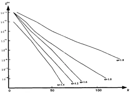
is the identity matrix and A is a dense matrix with random elements. Specifically, the elements of A and 8 were chosen from the intervals [-10,10] and [1,10], respectively, and I were set equal to -8. All elements of the constant vector XO in the objective function were set to be 10.

Closeness of an iterate J;(k) to the solution is measured in terms of the residual of the constraint inequalities of

P,

which is defined by

where ( . )+ = max{ " O}. Because of the primal-dual nature of the algorithm, x(k) is optimal whenever it is feasible to

P,

in which case r(k) vanishes.

Figure 1 illustrates how {r(k)} decreases as the iteration proceeds for a test problem with

(n, m) = (75,50). From the figure, we may observe that the algorithm is linearly convergent for any value of relaxation parameter w.

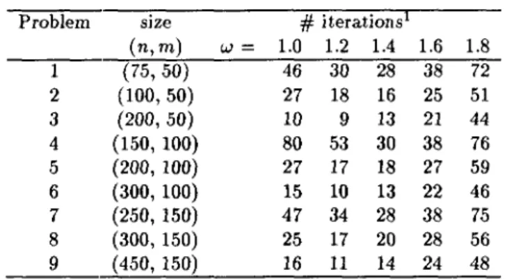
In order to see how the choice of parameter w affects the performance of the algorithm, we then solved several test problems of various sizes. The results are summarized in Table

1 ()-1 -2 11l -3 III

-.

10 o

Fig. 1. Behavior of the proposed algorithm

1, in which the numbers indicate how many iterations were required to attain the termination criterion

r(k) :::; 10-4 .

From Table 1, we see that the algorithm converges faster when w is chosen around 1.2 '" 1.4. It is noted that, when w = 1.0, the algorithm is nothing but the extended Hildreth's algorithm for solving interval constrained problems proposed by Lent and Censor [8]. 5.2 Parallel computation for transportation problems

Hildreth type algorithms are most effectively a.pplied to problems with sparse constraint matrix and the network flow problem is a typical example of such problems. Moreover, transportation problems are well suited to parallel implementation of Hildreth type algo-rithms, because of the bipartite network structure [12J.

In the numerical experiments, we have applied Algorithm 3.1 to the following trans-portation problem with quadratic cost function:

N s.t. LXij = Si, i = 1, ... ,M, j=1 M LXij

=

dj, j

=

1, ... ,N, i=1 0:::; Xij::; Uij, i = 1, ... ,M, j = 1, ... ,N.

Note that this class of problems has also been considered by Zenios and Censor [12], who implemented a Hildreth type algorithm on a massively parallel Connection Machine CM-2. In our experiments, we have implemented Algorithm 3.1 on a parallel computer called

88 Y. Shimazu, M Fukushima & T. Ibaraki

Table 1: Computational results for problem

P.

Problem size

#

iterationsl

(n,m) w= 1.0 1.2 1.4 1.6 1.8 1 (75,50) 46 30 28 38 72 2 (100, 50) 27 18 16 25 51 3 (200,50) 10 9 13 21 44 4 (150, 100) 80 53 30 38 76 5 (200, 100) 27 17 18 27 59 6 (300, 100) 15 10 13 22 46 7 (250, 150) 47 34 28 38 75 8 (300, 150) 25 17 20 28 56 9 (450, 150) 16 11 14 24 48 1 Termination criterion: r(k)

:s

10-4

Table 2: Computational results for transportation problems.

(M,N)

#

iterationsl CPU sec CPU sec serial2 _parallel3 (100, 100) 37 12.75 0.133 (200, 200) 33 47.14 0.201 (300,300) 35 114.48 0.698 (400, 400) 34 208.38 0.854 (500, 500) 34 328.44 1.054 (600, 600) 35 497.91 1.894 (700,700) 34 653.88 2.219

1 Termination criterion: max {maxi {12::j

xl;) -

Si

I} ,

maxj {12::i

xl;) -

dj

I} }

:S 10-.4

2 Serial computation implemented on SUN SPARe! IPX

3 Parallel computation implemented on ADENA

ADENA [7] at the Department of Applied Mathematics and Physics, Kyoto University. ADENA was originally designed to solve PDE's and consists of 16 x 16 PE array, i.e., 256 PEs. Its performance is estimated as 2.56 GFLOPS (peak) or 1.0 GFLOPS (effective). We also implemented the algorithm (serially) on a SUN SPARK1 IPX. By some prelimi-nary experiments, we have found that SUN SPARK IPX performs floating point arithmetic operations about 2 times fa~ter than a single processor element of ADEN A.

The results of both implementations are summarized in Table 2, which shows the num-bers of iterations and CPU times (sec.) for problems of various sizes with termination criterion

max{mrx{

~xl7)

-Si}

,mtx{!~xl7)

-dj

!}}

~

10-4.

The results strongly suggest that the proposed algorithm is amenable to parallel computation for this type of problems.

6 Conclusion

In this paper, we have proposed an SOR modification of Hildreth's algorithm for solving interval constrained quadratic programming problems. The proposed algorithm is shown to

converge at a linear rate. Our limited computational experience demonstrates the effective-ness of the proposed algorithm.

Acknowledgement We are indebted to the referees and Mr. Eiki Yamakawa of Advanced Telecommunications Research Institute International for careful reading of the manuscript. In particular, we are grateful to one of the referees who kindly pointed out that the rate of convergence results of Section 4.3, which were only proved for the special case Q

=

I in an earlier version of the paper, could be extended to the general case as shown in the finial versIOn.

References

[1] Bertsekas, D.P. and Tsitsiklis, J.N.: Parallel and Distributed Computation: Numerical Methods. Prent.ice Hall, New Jersey, 1989.

[2] Censor, Y.: Row-Action Methods for Huge and Sparse Systems and Their Applications. SIAM Review, Vol. 23 (1981),444-466.

[3] Censor, Y. and Lent, A.: An Iterative Row·Action Method for Interval Convex Pro-gramming. Journal of Optimization Theory and Applications, Vol. 34 (1981), 321-:353. [4] Herman, G.T. and Lent, A.: A Family of Iterative Quadratic Optimization Algorithms

for Pairs of Inequalities, with Application in Diagnostic Radiology. Mathematical Pro-gramming Study, Vol. 9 (1979), 15-29.

[5] Hildreth, C.: A Quadratic Programming Procedure. Naval Research Logistics Quar-terly, Vol. 4 (l!l57), 79-85.

[6] Iusem, A.N. and De Pierro, A.R.: On the Convergence Properties of Hildreth's Quadratic Programming Algorithm. Mathematical Programming, Vol. 47 (1990), 37-51.

[7] Kadota, H., Kaneko, K., Tanikawa, Y. and Nogi, T.: VLSI Parallel Computer with Data Transfer Network: ADENA. Proceedings of the 1989 International Conference on Parallel Processing, The Pennsylvania State University Press, Vol. 1 (1989), 319-322. [8] Lent, A. and Censor, Y.: Extensions of Hildreth's Row-Action Method for Quadratic

Programming," SIAM Journal on Control and Optimization, Vol. 18 (1980), 444-454. [9] Lin, Y.Y. and Pang, J.S.: Iterative Methods for Large Convex Quadratic Programs: A

Survey. SIAM Journal on Control and Optimization, VOl. 25 (1987), 383-411.

[10] Nielsen, S.S. and Zenios, S.A.: Massively Parallel Algorithms for Singly Constrained Nonlinear Programs. ORSA Journal on Computing Vol. 4 (1992), 166-181.

[11] Zenios, S.A. and Lasken, R.A.: Nonlinear Network Optimization on a Massively Parallel Connection Ma.chine. Annals of Operations Research, Vol. 14 (1988), 147-165.

[12] Zenios, S.A. and Censor, Y.: Massively Parallel Row-Action Algorithms for Some Non-linear Transportation Problems. SIAM Journal on Optimization, Vol. 1 (1991),373-400.

Masao FUKUSHIMA:

Graduate School of Information Science,

Advanced Institute of Science and Technology, Nara, Takayama, Ikoma, Nara 630-01, Japan