Virtual turning points and bifurcation of Stokes curves for higher order ordinary differential
equations
Takashi AOKI
1, Takahiro KAWAI
2, Shunsuke SASAKI
3, Akira SHUDO
4and Yoshitsugu TAKEI
51
Department of Mathematics, Kinki University Higashi-Osaka, 577-8502 Japan
2,3,5
Research Institute for Mathematical Sciences Kyoto University, Kyoto, 606-8502 Japan
4
Department of Physics, Tokyo Metropolitan University
Hachioji, Tokyo 192-0397 Japan
Abstract
For a higher order linear ordinary differential operatorP, its Stokes curve bifurcates in general when it hits another turning point ofP. This phenomenon is most neatly understandable by taking into account Stokes curves emanating from virtual turning points, together with those from ordinary turning points. This understanding of the bifurcation of a Stokes curve plays an important role in resolving a paradox recently found in the Noumi-Yamada system, a system of linear differential equations associated with the fourth Painlev´e equation.
Exact WKB analysis, that is, WKB analysis based on the Borel resum- mation, has turned out to be an important and useful tool in mathematical physics [1]; its advantage certainly consists in its efficiency in manipulating exponentially small terms, but still more important, from the theoretical view- point, are the fact that the Borel transform of an ordinary differential operator P(x, η−1d/dx) with a large parameterη is a partial differential operator on the (x, y)-space withy denoting the variable dual toη, and the fact that microlo- cal analysis, a new and powerful machinery in mathematics [2], clarifies the structure of singularities of solutions of the Borel transformed equation, i.e., the Borel transformed WKB solutions, which are multi-valued analytic functions on (x, y)-space. An important example of the influence of microlocal analysis on WKB analysis is the introduction of the notion of a virtual turning point for differential equations of the third or higher order [3]; it is, by definition, thex- component of the self-intersection point of a bicharacteristic curve of the Borel transform of the operatorP(x, η−1d/dx). Note that a bicharacteristic curve is the most “elementary” carrier of singularities of solutions of linear partial differ- ential equations in general [2]. Note also that Voros [4] uses the corresponding result for the Tricomi-type operator in constructing his theory of exact WKB analysis for differential operators of the second order. As the so-called new Stokes curve for higher order operators [5] is nothing but an ordinary Stokes curve emanating from a virtual turning point, the importance of the notion of a virtual turning point is practically evident. Actually it plays an important role in computing the transition probabilities for the non-adiabatic transition problem of the Landau-Zener type [6]. In this paper we show how important a role a virtual turning point plays from the theoretical viewpoint. To be more concrete, we validate the following Assertion A using a concrete example we encounter in the exact WKB analysis of the Painlev´e transcendent [7]:
Assertion A: The role of a virtual turning point is commensurate with that of an ordinary turning point; theoretically speaking, there is no distinction between them.
In validating this challenging assertion, we divide our discussion into two steps: we first show the mechanism that relates a virtual turning point with the bifurcation phenomenon of a Stokes curve that is observed when it hits a simple turning point, and then we argue how the mechanism works in understanding the true nature of a seemingly paradoxical phenomenon which has been just found [7].
The relevance of a virtual turning point and the bifurcation of a Stokes curve has been recognized since a couple of years ago [8], but it has not been published in literature.
We start with a third (or higher) order differential operatorP(x, η−1d/dx) with a large parameter η. Let us consider the situation where a Stokes curve emanating from a turning points1 hits another simple turning point s2. We further suppose that the Stokes curve is of type (1,2), i.e., an integral curve of the direction field
(1) Im(ξ1(x)−ξ2(x))dx= 0,
and thatx=s2satisfies
(2) ξ2(x) =ξ3(x),
where ξj(x) (j = 1,2,3) are mutually distinct solutions of the characteristic equation P(x, ξ) = 0. Here we have used the assumption that P is of third (or higher) order; in the case of operators of the second order, this situation cannot be observed. Now, sincex=s2 is a simple turning point whereξ2(x) andξ3(x) merge by the assumption (2),ξ2(x) (andξ3(x) also) has a square-root type singularity atx=s2 and the Stokes curve bifurcates there (Fig.1).
If the operatorP does not contain any parameter other thanη, one might be content to regard this bifurcation just as one of the pathologies which analysis of higher order equations presents. Then the reasoning would be stopped there.
But, if the operator P depends on an auxiliary parameter t, it is natural to consider how the configuration of Stokes curves changes as the parameter t changes. Then it is more reasonable to take into account the Stokes curve emanating froms2, in addition to the Stokes curve emanating froms1. To fix the situation, let us suppose their configurations are those given in Fig.2 (resp., Fig.3) fort =t2 (resp., t=t3). We also suppose that s2(t) lies on the Stokes curve emanating froms1(t) whent=t1. In the situation we observe in Fig.2, we know that there exists a virtual turning pointv=v(t) such that a Stokes curve of type (1,3) emanating fromv passes through the crossing point of the Stokes curve emanating froms1 and that froms2[8] (cf. Fig.20). The configuration of these Stokes curves then becomes as described in Fig.30 whent=t3in all cases we have examined [9]. Since the Stokes curve emanating fromv(t1) is of type (1,3), it also bifurcates ats2(t1) because of the singularity thatξ3(x) contains.
The resulting configuration is given in Fig.10. Comparing Figures 10, 20 and 30, one naturally observes that the configuration of Stokes curves continuously changes as the parametertmoves, in spite of the fact that the relative location of the Stokes curve emanating from v(t) and that from s1(t) is interchanged on the right of their crossing points. Thus we can understand the bifurcation of a Stokes curve to be a natural counterpart of the addition of a Stokes curve emanating from a virtual turning point; it is not an isolated pathology! We refer the reader to [9] for the concrete description of Stokes curves in the example of the Stokes geometry for the quantized H´enon map.
We now show how the mechanism described above is related to the paradox- ical situation which one of us (S.S.) has recently found [7] in the computer- assisted study of the Stokes geometry of the Painlev´e hierarchy of Noumi- Yamada type [10]; its first member, with which we are concerned in this paper, consists of the following symmetric form of the fourth Painlev´e equation [11]
(3) η−1dfj
dt =fj(fj+1−fj+2) +αj (j = 0,1,2)
with fj = fj−3 (j = 3,4) and α0 +α1 +α2 = η−1, and its underlying
“Schr¨odinger” equation (4)
−η−1x ∂
∂x
ψ0
ψ1
ψ2
=
(2α1+α2)/3 f1 1 x (−α1+α2)/3 f2
xf0 x −(α1+ 2α2)/3
ψ0
ψ1
ψ2
together with its deformation equation
(5) η−1∂
∂t
ψ0
ψ1
ψ2
=
f2− t
2 −1 0
0 f0− t
2 −1
−x 0 f1− t 2
ψ0
ψ1
ψ2
.
As is well-known, the equation (3) is nothing but the compatibility condition of the equations (4) and (5). As the equation (3) is equivalent to the fourth Painlev´e equation, we can use more traditional pair of the “Schr¨odinger” equa- tion and its deformation equation [12] so that their compatibility condition is equivalent to (3). Actually in the traditional case the “Schr¨odinger” equation is of the second order. Now, one of the results of [13] asserts that, if the parameter tlies on the Stokes curve of (3) (to be more precise, the appropriate linearization of (3); see [13] for the details), two turning points of the “Schr¨odinger” equation are connected by a Stokes curve of the “Schr¨odinger” equation. On the other hand, a computer-assisted study of the Stokes geometry of the equations (3) and (4) shows the following intriguing fact [7] (here we have chosenα0= 1.0 + 0.6i andα1= 0.2−0.1i):
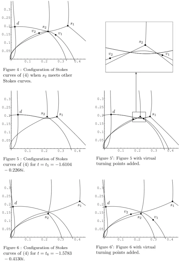
If the parametertis on the Stokes curve of (3) and if it is sufficiently close to its origin, i.e., a turning point of (3), then a double turning pointdand a simple turning points1 of equation (4) are connected by a Stokes curve of (4) (Fig.5;
here we have included another simple turning points2 for the later reference).
However, whent lies in some portion, sayσ, of the same Stokes curve which is far away from the turning point of (3), no pair of turning points of equation (4) are connected by a Stokes curve of (4), unless virtual turning points are counted as turning points (Fig.6; we have also included the simple turning points2 in this figure).
One might be puzzled by the apparent contradiction between the above quoted result of [13] and the latter half part of the observation of [7], namely,
the fact that no pair of turning points of (4) is connected by a Stokes curve of (4) for the parameter t in the portion σ of a Stokes curve of (3). As we see below, this paradox is resolved in a natural manner if a virtual turning point is counted as a turning point.
Let us first note, by comparing Fig.5 and Fig.6, that the Stokes curve con- necting turning pointsdands1should hit the turning points2as the parameter tmoves from the portion close to the turning point of (3) (i.e., generating Fig.5) to another portionσof the Stokes curve of (3) that is far away from the turning point (i.e., generating Fig.6). Hence it is reasonable to surmise that bifurcation of a Stokes curve should occur in the course of the journey oft from a point, sayt5, giving rise to the configuration of Stokes curves of (4) in Fig.5, and to another point, say t6, giving rise to Fig.6. As we know that the bifurcation phenomenon is a counterpart of the addition of Stokes curves emanating from virtual turning points, we include virtual turning points in Fig.5 to find Fig.50. Since we have two kinds of crossing points of Stokes curves, i.e., the crossing of the Stokes curve emanating froms1 and that froms2, and the crossing of the Stokes curve froms2 and that from d, we write in two virtual turning points v1 and v2. (We have omitted some other virtual turning points which are not of our immediate concern.) In parenthesis, an interesting fact worth mention- ing is that v1 and v2 are connected by a Stokes curve. As t moves from t5
to t6, we should encounter the configuration of Stokes curves given in Fig.4.
In Fig.4 the virtual turning pointv1 is connected with both the double turn- ing point d and the virtual turning point v2 thanks to the bifurcation of the Stokes curve emanating fromv1, and similarly the virtual turning point v2 is connected with both the simple turning points1 and the virtual turning point v1. Whentmoves further to reacht6, the interchange of relative location of the Stokes curve emanating fromv1 and that froms1 on the left of their crossing point switches the target of the Stokes curve (emanating fromv1) from v2 to the double turning pointd. In parallel with this, the target of the Stokes curve emanating fromv2 becomess1, notv1. Thus we obtain Fig.60, wheres1(resp., d) in Fig.5 is superseded byv1(resp.,v2), that is, virtual turning pointsv1and v2 are respectively connected by a Stokes curve with ordinary turning pointsd and s1 but d and s1 are not connected. Thus we clearly see that a “virtual”
turning point is really a “real” object even though not “ordinary”. (From the viewpoint of the topological complexity, Fig.50 corresponds to Fig.30 and Fig.60 corresponds to Fig.20. Hence it might be better, logically speaking, to arrange our argument so that we may start fromt=t6 and reacht=t5. Here we have arranged the materials so that we may start with a “usual”situation and end up with an “unusual” situation with the change of the parameter.)
In conclusion, we emphasize that virtual turning points and (ordinary) turn- ing points play equal roles in Fig.60, validatingAssertion A.
In ending this paper we note that the geometric study given here strongly indicates that connection formula for the wave functionψ=t(ψ0, ψ1, ψ2) (i.e., a solution of (4)) across a Stokes curve emanating from a virtual turning point should be relevant to the connection formula for the Painlev´e transcendents. It should be an important and interesting problem to study in general how the
analytic structure of the wave function near a Stokes curve emanating from a virtual turning point is related to the connection formula for the novel tran- scendents that appear as solutions of a higher member in the Noumi-Yamada hierarchy, i.e., the so-called higher order fourth Painlev´e equation.
Acknowledgment: The research of the authors has been supported in part by JSPS Grant-in-Aid No.14340042, No.14077213, No.15540190 and No.16540148.
References
[1] C. M. Bender and T. T. Wu, Phys. Rev.,184, 1231 (1969), A. Voros, Ann. Inst. Henri Poincar´e, 39, 211 (1983), J. Zinn-Justin, J. Math. Phys., 25, 549 (1984), H. J. Silverstone, Phys. Rev. Lett.,55, 2523 (1985),
E. Delabaere, H. Dillinger et F. Pham, Ann. Inst. Fourier,43, 433 (1993), T. Kawai and Y. Takei, Algebraic Analysis of Singular Perturbations.
(Iwanami, 1998. In Japanese and its translation will be published by AMS in 2004).
[2] L. H¨ormander, Acta Math.,27, 79 (1971),
M. Sato, T. Kawai and M. Kashiwara, Microfunctions and pseudo- differential equations, Lect. Notes in Math., No.287, pp.265-529 (1973).
[3] T. Aoki, T. Kawai and Y. Takei, in Analyse alg´ebrique des perturbations singuli`eres. I. (ed. by L. Boutet de Monvel), Hermann, pp.69-84 (1994). A virtual turning point is called a new turning point in this article.
[4] A. Voros, in Ref.[1].
[5] H. L. Berk, W. M. Nevins and K. V. Roberts, J. Math. Phys., 23, 988 (1982).
[6] T. Aoki, T. Kawai and Y. Takei, J. Phys.,A35, 2401 (2002).
[7] S. Sasaki (to be published).
[8] T. Aoki, T. Kawai and Y. Takei (unpublished), A. Shudo and K. S. Ikeda (to be published).
[9] A. Shudo and K. S. Ikeda, in Ref.[8].
[10] M. Noumi and Y. Yamada, Funkcialaj Ekvacioj,41, 483 (1998).
[11] V. E. Adler, Physica,D37, 335 (1994).
[12] K. Okamoto, J. Fac. Sci. Univ. Tokyo, Sect.IA,33, 575 (1986).
[13] T. Kawai and Y. Takei, Adv. in Math.,118, 1 (1996), and the article in Ref.[1].
s
1s
2s
1s
2v
Figure 1 : Bifurcation of a Stokes curve. Figure 10: Figure 1 with a virtual turning point added.
s
1s
2s
1s
2v
Figure 2 :Configuration of Stokes curves fort=t2.
Figure 20: Figure 2 with a virtual turning point added.
s
1s
2s
1s
2v
Figure 3 : Configuration of Stokes curves fort=t3.
Figure 30: Figure 3 with a virtual turning point added.
0.1 0.2 0.3 0.4 0.05
0.1 0.15 0.2 0.25 0.3
d s2 s1
v1
v2
s2
v2 v1
6 Figure 4 : Configuration of Stokes
curves of (4) whens2 meets other Stokes curves.
0.1 0.2 0.3 0.4
0.05 0.1 0.15 0.2 0.25 0.3
0.1 0.2 0.3 0.4
0.05 0.1 0.15 0.2 0.25 0.3
d s2 s1 d s1
Figure 5 : Configuration of Stokes curves of (4) fort=t5=−1.6104
−0.2268i.
Figure 50: Figure 5 with virtual turning points added.
0.1 0.2 0.3 0.4
0.05 0.1 0.15 0.2 0.25 0.3
0.1 0.2 0.3 0.4
0.05 0.1 0.15 0.2 0.25 0.3
d
s2
s1 d s1
s2 v1
v2
Figure 6 : Configuration of Stokes curves of (4) fort=t6=−1.5783
−0.4130i.
Figure 60: Figure 6 with virtual turning points added.