選択実験における一般化多項ロジットのサブクラスの予備的検討

(1)

実践論文

選択実験における一般化多項ロジットのサブクラスの予備的検討

フェアトレード・カップコーヒーに関する日本の大学生調査データを事例として

Preliminary Examination of Generalized Multinomial Logit Subclasses on Choice Experiments

- Japanese Undergraduate Survey Data on a Takeaway Cup of Fair Trade Coffee -

大床太郎^*1

Taro Ohdoko

Email: [email protected]

キーワード：多項ロジット; 混合ロジット; スケール不均一性多項ロジット; 一般化多項ロジット

Keywords: Multinomial Logit; Mixed Logit; Scale Heterogeneity Multinomial Logit; Generalized Multinomial Logit

環境の経済評価において選択実験が頻繁に用いられるようになった一方で，選好とスケールの多様性に関する課題を含む多くの研究課題が残されている．近年，

Fiebig et al. (2010)

によって，選好とスケールの多様性の双方を含むことのできる一般化多項ロジット（generalized multinomial logit: GMNL）が開発された．

GMNL

は，多項ロジット，混合ロジット，スケール不均一性多項ロジット，一般化多項ロジットタイプ

I

とタイプ

II

をすべてプロシージャーのサブクラスとして包含できる離散選択モデルである．フェアトレード・カップコーヒーに関する日本の大学生を回答者とする選択実験データを用いて，すべてのサブクラスを比較したところ，GMNLは対数尤度を改善した一方で，的中率やモデル適合性の観点で他のサブクラスに劣りうることを予備的に確認した．

While choice experiment techniques are being applied increasingly in many environmental valuation situations, there are a number of methodological issues to be resolved, such as preference and scale heterogeneity. Fiebig et al. (2010) developed a generalized multinomial logit (GMNL) model to incorporate both preference and scale heterogeneity into a model. The GMNL model includes multinomial or conditional logit, mixed or random parameter logit, scale heterogeneity logit, and GMNL type I and type II into one model as subclasses of the procedure. Here, we examine the prediction success of these subclasses. Using Japanese undergraduate choice experiment data on a takeaway cup of fair trade coffee, the GMNL model improved the value of the log likelihood; however, the model performance, including the hit rate and model-fit measures, was inferior to the other subclasse.

―――――――――

*1:

獨協大学経済学部

(2)

1. Introduction

There has been growing interest in eliciting preferences or willingness to pay (WTP) for marketing and policy-making purposes. Two methods are used to elicit preferences, namely revealed preferences and stated preferences (Louviere et al.

⁽⁴⁰⁾

). The revealed preferences method, which includes a hedonic price function, has high reliability because it utilizes behavioral data in existing markets. However, it suffers from multicollinearity between covariates, relatively poor flexibility because it analyzes existing alternatives, and relatively low data availability frequency. On the other hand, the stated preference method, which includes choice experiments (CE), describes hypothetical behavior such that it has relatively high flexibility and can cope with multicollinearity by using certain experimental design procedures. It also

“seems to be reliable when respondents understand, are committed to and can respond to tasks”

(Louviere et al. P.24

⁽⁴⁰⁾

). CE can assess several variables simultaneously, in such a way that the preferences for options that consist of several attributes are clarified.

A discrete choice model, known as a generalized multinomial logit (GMNL) model, has been developed to cope with several heterogeneous responses (Fiebig et al.

⁽¹⁹⁾

). This model can simultaneously analyze preference heterogeneity and scale heterogeneity, which can describe differences in preference certainty across individuals.

Moreover, because the GMNL model contains the subclasses of multinomial logit (MNL; McFadden

(49)

), random parameter or mixed logit (MIXL;

Revelt and Train

⁽⁵³⁾

), scale heterogeneity logit (S- MNL), and GMNL type I (GMNL-I) and type-II (GMNL-II), five models can be examined in an integrated manner. The GMNL model has thus

attracted considerable attention in CE studies in an attempt to model responses precisely and correctly.

However, there have been mixed results with regard to the application of GMNL in CE studies.

Some studies (e.g., Goossens et al.

⁽²⁴⁾

) did not use GMNL because of poor model fit compared with other discrete choice models. Although the application of GMNL is generally favored by CE researchers and practitioners, we should examine the advantages and disadvantages of applying GMNL to CE data.

There are several ways to compare the GMNL model with other discrete choice models. We utilized the hit rate, which is the level of prediction success achieved by using the estimated parameters. In addition, we compared the measures of model fit, which consist of McFadden’s ρ modified by the degree of freedom and compared with a no- coefficients model and a constants-only model, and the value of log-likelihood, which has been frequently employed in CE studies. For all of these measures, we compared GMNL with MNL, MIXL, and S-MNL for a preliminary examination of the GMNL subclasses.

The remainder of the paper is organized as follows. Section 2 reviews the relevant literature.

The dataset and the econometric methods employed are presented in Section 3, with results and discussion in Section 4. Concluding remarks, including topics for future research, are provided in Section 5.

2. Literature Review

We utilized CE data from Japanese undergraduates

at Dokkyo University and employed a takeaway cup

of fair trade coffee as the evaluated object. In

addition, we employed the international fair trade

label FAIRTRADE in the choice sets of the CE. We

(3)

first review the GMNL model and relevant studies and then the CE with labels and fair trade.

2.1. The GMNL Model in CE Studies

Along with the growing use of CE techniques, increasing attention has been paid to the analysis of CE data. The traditional MNL assumed preference homogeneity and that preferences were independent of irrelevant alternatives (IIA). Two alternative models were frequently employed to incorporate preference heterogeneity and to overcome the need to assume the IIA property, namely a random parameter or MIXL (Revelt and Train

⁽⁵³⁾

, Train

⁽⁶²⁾

, among others) and a latent class model (Boxall and Adamowicz

⁽⁸⁾

, Shonkwiler and Shaw

⁽⁶⁰⁾

, Greene and Hensher

⁽²³⁾

, among others). The former allows for a continuous distribution of preferences, whereas the latter allows for a discrete distribution.

However, there is an underlying issue that is inherent in the use of the random utility model (RUM), namely a scaling problem. A RUM assumes that the indirect utility function associated with alternatives of CE questions is U V X ε , where n 1, ⋯ , N denotes the respondents;

j 1, ⋯ , J is the alternatives in the choice set; t 1, ⋯ , T is the choice occasion; X is the matrix of attributes of the alternatives; and ε is the error component. The observable component of indirect utility, V X , has been frequently specified in an additively separate form, β X , where β denotes the marginal utility vector, which we also utilized.

However, it has been demonstrated that the ‘true’

marginal utility vector, β , is confounded with the scale parameter, λ, which is inversely proportional to the variance of the error component, such that β βλ (Louviere et al.

⁽⁴⁰⁾

). For example, Louviere and Eagle

⁽³⁸⁾

argued that the model should be developed to distinguish preference heterogeneity and scale heterogeneity. A critical issue has been

whether respondents’ heterogeneous features are included in their preferences, or scales, or both.

Fiebig et al.

⁽¹⁹⁾

developed the GMNL model, after Keane

⁽²⁹⁾

first presented a relevant research program. Fiebig et al.

⁽¹⁹⁾

incorporated two parameters in the discrete choice model so that preference heterogeneity and scale heterogeneity could be analyzed simultaneously. They demonstrated that the GMNL model was preferred in seven out of the 10 datasets that they analyzed. For the other three datasets, the preferred model was S- MNL, which is a subclass of the GMNL model and incorporates only scale heterogeneity with fixed preference parameters.

The GMNL model is being increasingly applied in choice modeling (CM), which includes CE, best–worst scaling (BWS) studies (Louviere et al.

⁽³⁹⁾

). Knox et al.

⁽³¹⁾

utilized GMNL in CE and scenario framing, or the information effect, on prescribed contraceptive products, where they succeeded in improving the empirical results by using GMNL. Czajkowski et al.

⁽¹³⁾

applied a GMNL model to a CE study of forest ecosystem management in Poland, which demonstrated that the GMNL model had an enhanced model fit compared with MIXL. Li et al.

⁽³⁶⁾

applied a GMNL model to a CE study of refrigerator purchases by consumers, where the CE question included a voluntary climate action program by the manufacturer as an attribute.

They demonstrated that the GMNL model had an

enhanced model fit compared with the MNL and

MIXL models. Doiron et al.

⁽¹⁷⁾

applied a GMNL

model to a BWS study on the job choices of student

nurses and demonstrated that the GMNL model had

an enhanced model fit compared with the MNL and

MIXL models. In contrast, Greene and Hensher

⁽²²⁾

demonstrated that scale heterogeneity might not

improve the empirical results with regard to direct

elasticity and WTP by utilizing transportation mode

choice data, and Goossens et al.

⁽²⁴⁾

could not

(4)

improve their empirical results from CE on early assisted discharge of chronic obstructive pulmonary disease patients to home. Nevertheless, the GMNL model appears to become gradually the standard discrete choice model that expresses respondents’

choices correctly and precisely.

2.2. CE with Labels and Fair Trade

Multiple labeling has been researched extensively in the context of CE on food. For example, nutritional facts or health claims have been examined in numerous studies (Barreiro-Hurle et al.

⁽⁴⁾

; Drescher et al.

⁽¹⁶⁾

; Gao and Schroeder

⁽²¹⁾

; Lacanilao et al.

⁽³⁵⁾

; Lowe et al.

⁽⁴¹⁾

; Lusk and Parker

⁽⁴³⁾

; Hu et al.

⁽²⁷⁾

; Mørkbak et al.

⁽⁵⁰⁾

), as has genetically modified product labeling (Burton and Pearse

⁽⁹⁾

; Kontoleon and Yabe

⁽³²⁾

; Rigby and Burton

⁽⁵⁴⁾

; Carlsson et al.

(10)

; Tonsor et al.

⁽⁶¹⁾

; Volinsky et al.

⁽⁶⁴⁾

). Many studies have used organic labels or sustainability labels (Aizaki et al.

⁽¹⁾

; Fonner and Sylvia

⁽²⁰⁾

; Hu et al.

⁽²⁷⁾

; Mauracher et al.

⁽⁴⁶⁾

; Onozaka and McFadden

(51)

; Rigby and Burton

⁽⁵⁴⁾

; Scarpa et al.

⁽⁵⁹⁾

; van Loo et al.

⁽⁶³⁾

); labels related to health risk or safety have also been studied (Aizaki et al.

⁽¹⁾

; Imami et al.

⁽²⁸⁾

; Kontoleon and Yabe

⁽³²⁾

; Mørkbak et al.

⁽⁵⁰⁾

). Most of these studies have demonstrated the positive effect on consumer choice of certain labeling, and it can be supposed that some simple food labels may provide reputational information (Scarpa et al.

⁽⁵⁹⁾

; Bonaiuto et al.

⁽⁶⁾

) that helps consumers to choose with confidence, which may alleviate “information overload” (Malhortra

⁽⁴⁵⁾

).

Regarding the fair trade label, Onozaka and McFadden

⁽⁵¹⁾

conducted CE surveys on consumer choice of Gala apples and red round tomatoes through a national web-based survey in the USA. As CE attributes, they included product origin, certified organic, certified fair trade, carbon footprint, and price. From the results of a MIXL model, they found

that certified fair trade evaluates positively in both products; locally grown is the most valued and its value is enhanced with fair trade certification for red round tomatoes. They discriminated between labels such as fair trade and organic. They defined fair trade certification as domestic. De Pelsmacker et al.

⁽¹⁵⁾

estimated WTP for fair trade coffee in Belgium using CE, and suggested that there is a 10% price premium to the fair trade label, where they only used the fair trade label. They designated fair trade as “a label on the package (that) indicates that a fair price for the coffee harvest is guaranteed to the farmers of the South”, which is relevant to developing countries in Global South. Cicia et al.

⁽¹¹⁾

demonstrated that Italian consumers were willing to pay a positive price premium for fair trade coffee using CE, where they distinguished the fair trade label from the fair trade plus organic label, and also focused on developing countries. Cranfield et al.

⁽¹²⁾

showed a positive price premium paid by Canadian consumers from CE data, where they examined organic claims, labeled fair trade, and certified fair trade. The premium was higher for certified fair trade than for the label, with a focus on developing countries in South America. Rotaris and Danielis

⁽⁵⁵⁾

showed a positive price premium for a fair trade label in the Italian market using CE, focusing on developing countries. In addition, Lusk and Briggeman

⁽⁴²⁾

, using BWS data, suggested that there are positive correlations between preferences for fairness, which they defined as “the extent to which all parties involved in the production of the food equally benefit”, and reported the WTP for organic bread.

However, to our knowledge, little research has been conducted on fair trade labeling that includes information on both geographical area and what the producers use the revenue from their fair trade products for.

3. Materials and Methods

(5)

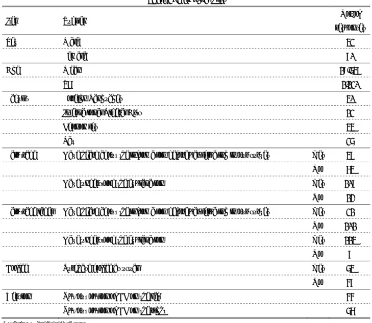
We administered our survey at Dokkyo University from April 12 to 29, 2016. Before implementation, we conducted preliminary discussions with eight undergraduates attending a seminar course given by Dr. Ohdoko on the design of the questionnaire and the selection of the attributes of the CE questions; we then conducted a pretest session to improve the quality of the questionnaire using 16 other undergraduates attending the seminar course. We implemented the in-person self-administered CE survey to elicit the preferences for the attributes of a takeaway cup of coffee such as one might purchase from Starbucks. Indeed, there is a coffee shop at Dokkyo University that serves takeaway cups of coffee. The attributes included the geographical area in which the coffee was grown, what the producers use the revenue from their fair trade products for, and the price.

We then selected the levels of attributes (Table 1). For the geographical area in which the coffee was grown, we selected Africa, Asia, and South America, which were assumed to be familiar to Japanese undergraduates as origins of coffee and/or the location of developing countries supported by developed countries. For the revenue mainly used for, we selected three levels to mimic the actual situation of Fairtrade International’s standards

¹

: support in developing countries mainly for workers’ autonomy, human rights and education especially for women and children, and traditional agricultural practices to protect the environment of developing countries. For price, we selected levels to mimic the actual situation in the Japanese market for a takeaway cup of coffee.

Because the performance of a CE depends on respondents correctly interpreting the questionnaire, we simplified our questionnaire to make it as clear as possible.

1

http://www.fairtrade.net/ (retrieved December 13, 2016).

2

http://www.fairtrade-jp.org/ (retrieved Dec 13, 2016).

We organized our questionnaire as follows.

First, we collected demographic variables, including sex, age, and faculty at Dokkyo University. Second, we obtained information on fair trade, including its definition and the fair trade label of Fairtrade International in accordance with the Fairtrade Japan website

²

. We then asked respondents whether they had heard about these before participating in our survey and whether they understood our explanations. Third, we provided our hypothetical scenario (see the Appendix) and nine CE questions;

we began with a sample question (Q0) and answer to ensure our respondents fully understood how to respond to our nine questions. Finally, we determined whether the respondents normally purchased cups of coffee and whether they believed in responsible business practices by employing likert scales in Arli and Lasmono

⁽³⁾

.

In creating the CE choice sets, we eliminated any possible correlation with the attributes in the experimental design methodology, primarily by using the main effects of a fractional factorial design along with the attributes and levels given in Table 1 to reduce the number of combinations below the maximum factorial 3

³

= 27 (Lorenzen and Anderson

(37)

). We created nine profiles, and randomly selected two of these to create our choice sets. For simplicity, we fixed the attribute order from top to bottom. An opt-out option was included to make it possible to mimic real-world situations (Ryan and Skåtun

⁽⁵⁶⁾

).

Thus, we provided two alternatives and one opt-out option for each CE question, which represented nine choices per respondent in accordance with the incorporation of a “too close to call option”

(Fenichel et al.

⁽¹⁸⁾

)

³

. In addition, we attached the international fair trade label with the permission of Fairtrade Japan at the top of all alternatives except the opt-out options. We sampled as many

3

Because it is difficult to translate “too close to call” in

Japanese, we used “I cannot choose between the two

alternatives.”

(6)

undergraduates as possible using convenience sampling and campus street intercepts. We distributed our nine CE survey questionnaires to 240 undergraduates, and we obtained 225 responses, of which 122 completed our questionnaire creating 1,058 useful CE observations. Table 2 shows the demographics of our sample, and Table 3 shows the respondents’ attitudes, as well as the results of our principal component analysis (PCA)

⁴

.

In their GMNL model, Fiebig et al.

⁽¹⁹⁾

first assumed the following random utility model:

U V X ε βλ X ε [Eq. 1],

where ε is the error component that depends on the Type I extreme value distribution; and λ π ⁄ 6σ is the scale parameter, which is inversely proportional to the variance of the error component, σ . Second, they extended the utility function to incorporate heterogeneities of both the marginal utility vector and the scale parameter, as follows:

U βλ γη 1 γ λ η X

ε [Eq. 2],

where η denotes the standard deviation of the marginal utility. The parameter γ is set to consider two GMNL models below. Then, the choice probability of the respondents becomes:

P j|X ; Β, Λ P U U , ∀k j

∬ ∏ exp β λ ′X /

∑ exp β λ ′X f β|Β f λ|Λ dβdλ [Eq. 3].

Simulated maximum likelihood estimation is employed (Train 2009).

Several different logit models can be estimated within our GMNL. When γ 1 , then β βλ η , which leads to GMNL-I, which assumes that the scale parameter affects only the mean marginal utilities. When γ 0 , then β

β η λ , which is GMNL-II and denotes that the

4

To utilize every covariate of the respondents, we employed only fully answered responses. We used the procedure

“princomp3,” which is a modification of the “princomp”

procedure in R, to conduct a “varimax” rotation and produce

scale parameter affects both the mean and the standard deviation of the marginal utilities. When η 0 ∀n , then β βλ , and we have S-MNL, which assumes that the marginal utilities are identical between individuals, but that the scale parameter is distributed across individuals such that some preference uncertainty exists. When the variance of λ falls to zero, and the expectation of λ is set to unity, then, β β η , and the model reduces to MIXL, which assumes that only the marginal utilities are distributed across individuals.

Finally, when η 0 and the variance of λ falls to zero, then β β, and the model reduces to MNL.

As λ is proportional to the variance of the error term of utility, σ , it should be positive.

Fiebig et al.

⁽¹⁹⁾

transformed it exponentially as λ exp λ δ h τv , such that 0 ∝ 1 σ ⁄ , where h denotes sample covariates, and v , which is a random variable, depends on a standard truncated normal distribution, which we truncated at 2 such that 0 λ ∞ . The expectation of exponentially transformed λ should be standardized to unity to identify the marginal utility vector, such that E λ exp λ δ h τ /2 1. Fiebig et al.

⁽¹⁹⁾

imposed not only the expectation of λ but the mean, λ, set to unity in the simulated draws, which we followed.

The covariates of individuals can be incorporated into not only the scale parameter, such that λ exp λ δ h τv , but also the observable component of the indirect utility as the cross terms with the attributes of alternatives, such that h X . The parameters of these cross terms can be interpreted as the mean point estimate of the individual differences of the marginal utilities. We incorporated the demographic covariates in Table 2 and principal component scores of the attitudinal

principal component loadings directly (Aoki

⁽²⁾

). Cf. Shigenobu

Aoki’s website: http://aoki2.si.gunma-u.ac.jp/ (in Japanese only,

retrieved September 30, 2015).

(7)

variables in Table 3 into both the cross term of the marginal utility and the covariates of the scale parameter.

In addition, Fiebig et al.

⁽¹⁹⁾

suggested that the alternative-specific constants (ASCs) should not be scaled, which we also followed

⁵

. In addition, because we included cross terms of the covariates with not only the attributes but also the ASCs, we decided not to scale the cross terms of the ASCs.

Although we can estimate the parameter γ directly, we assumed it lies between zero and one ( 0 1 ). Fiebig et al.

⁽¹⁹⁾

proposed a logistic transformation of γ estimating it indirectly as γ exp γ

^∗

⁄ 1 exp γ

^∗

. Indeed, in our preliminary estimations of S-MNL, the procedures became unstable when estimating γ directly, and it became more stable by indirect estimation. We thus decided to employ an indirect estimation procedure of γ.

We employed R 3.2.5 (R Core Team

⁽⁵²⁾

) and the procedure “gmnl” (Sarrias and Daziano

⁽⁵⁸⁾

) to estimate the GMNL model. We assumed that the distribution of η was normal, lognormal, uniform, or triangular. Greene and Hensher

⁽²²⁾

developed an alternative estimation procedure of  to ensure a smooth estimation. However, we ignored their procedure and instead concentrated on the acceptance/rejection random draws procedure of Fiebig et al.

⁽¹⁹⁾

. To test for an opt-out positional effect, we split our sample into two subsamples: one where the opt-out option was positioned on the left side and the other where the opt-out option was positioned on the right (Fig.1 and Fig. 2,

5

Fiebig et al. suggested that when we scaled ASCs, “(1) the estimates often ‘blow up,’ with  taking on very large values and the standard errors of the elements of  becoming very large; and (2) the model produces a substantially worse fit than one where only the coefficients on observed attributes are scaled, whereas ASCs are assumed homogenous in the population”. Indeed, our preliminary examination of ASC-scaled models suggests that such blown-up features are also present in our case.

6

When the level of the qualitative variable is l 1, ⋯ , L, and the arbitrarily omitted level is L , then the parameter of the omitted level, β , is estimated by the negative sum of the parameters of the remaining levels: β ∑ β .

respectively). When setting the ASCs, we set the left option of the opt-in options as ASC1, and the right option as ASC2. The opt-out option is not preferred when every ASC is positively and significantly estimated. We employed effects coding for the qualitative variable in our choice sets so as not to confound the ASCs and base level of the attributes of alternatives (Louviere et al.

⁽⁴⁰⁾

; Bech and Gyrd- Hansen

⁽⁵⁾

)

⁶

, while we assumed the price variable is continuous.

In searching for the best fit for the GMNL model, we employed a stepwise regression procedure with forward selection, judged by the Bayesian information criterion (BIC)

⁷

. First, we decided to incorporate all the mean marginal utility parameters of the attributes in the CE choice sets with the ASCs. In estimating GMNL, we first estimated which marginal utility parameters should be represented as normal, log-normal, uniform, or triangular to be best estimated by the GMNL. Then, we estimated it stepwise including the standard deviation parameters of the marginal utilities, cross terms of attributes and covariates, and covariates into the scale parameter, one by one. In estimating S- MNL, we first estimated the simple S-MNL that does not include any covariates, and we estimated it stepwise including the standard deviation parameters of the marginal utilities, cross terms of attributes and covariates, and covariates into the scale parameter, one by one. In estimating MIXL, we first estimated which marginal utility parameters should be represented as normal, log-normal, uniform, or

7

Fiebig et al.

⁽¹⁹⁾

concluded that “both BIC and CAIC (corrected

Akaike information criterion) provide accurate guides for

whether scale heterogeneity is present,” while “AIC (Akaike

information criterion) correctly picks models where errors are

correlated.” Although we should employ several criteria such as

BIC and CAIC, we decided to employ BIC. Indeed, the results

of MNL, MIXL, and S-MNL showed that the model selected by

BIC produced the highest hit rate rather than the models selected

by AIC, AIC3, or CAIC. In addition, our GMNL results did not

converge when selecting the model with AIC, AIC3, or CAIC.

(8)

triangular. Then, we estimated it stepwise including the standard deviation parameters of the marginal utilities or cross terms of attributes and covariates, one by one. In estimating MNL, we first estimated the simple MNL that does not include any covariates, and we estimated it stepwise including the cross terms of attributes and covariates.

In all the above cases, we utilized the 100 Halton draw sequence (Train

⁽⁶²⁾

). Then, we compared the results of each subclass of GMNL using three measures. First, we employed values of log likelihood. Second, we employed McFadden’s ρ modified by the degrees of freedom and compared it with a no-coefficients model and a constants-only model, where the latter was estimated by MNL with only two ASCs. Third, we defined the hit rate as the measure of prediction success as follows: 1) we estimated values of the observable component of the indirect utilities using the mean parameter estimates of the mean marginal utilities; 2) we assigned a value of zero to the indirect utility of the opt-out option; 3) we compared the values of the indirect utilities in each choice set for each individual; 4) we predicted the choices of the individuals in each choice set; and then 5) we calculated the ratio between the number of prediction successes and the number of observations of choices on the CE. Although we may have to utilize individual parameters in MIXL, S-

MNL, and GMNL (Train

⁽⁶²⁾

; Fiebig et al.

⁽¹⁹⁾

), we utilized the procedure above for simplicity.

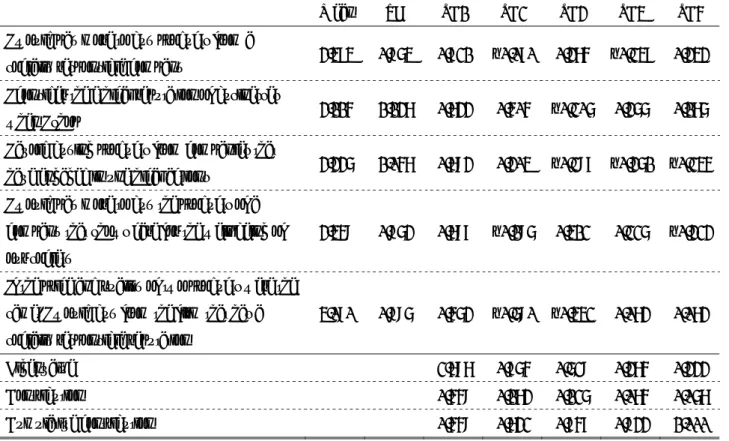
4. Results and Discussion

First, we interpret the results of our PCA on attitudinal variables in Table 3. When choosing components, we checked eigenvalues in excess of 1.000. As a result, we obtained one principal component (PC1 in Table 3). Then, we decided to interpret principal components with absolute values of component loadings in excess of 0.400. We interpret PC1 as indicating a preference for the products of ethical companies.

We present our list of variables in Table 4, and

estimated results in Table 5. Every subclass model

converged successfully. First, the value of log

likelihood is the largest in GMNL. Second, MIXL

enjoyed the highest hit rate; thus, the prediction of

respondents’ choice is best in MIXL, rather than the

other subclasses of GMNL. Third, McFadden’s ρ

also demonstrated that MIXL has the best fit among

the subclasses. We conclude that GMNL is not the

preferred model to describe respondents’ choice,

although the scale parameter, τ, and the weighting

parameter of GMNL, γ, increase the value of the log

likelihood.

(9)

Table 1: Attributes and Levels of Our CE Question

Attributes Level 1 Level 2 Level 3

Product origin South America Africa Asia

Revenue mainly used for Workers’ autonomy Human rights and education

Traditional agricultural practices

Price JPY280 JPY350 JPY420

Label

I cannot choose between the two alternatives

Product origin Asia South America

Revenue mainly used for Traditional agricultural

practices

Human rights and education

Price JPY 350 JPY 420

□ □ □

Fig. 1: Example of Choice Set with Left Opt-Out.

Label

I cannot choose between the two alternatives

Product origin Asia South America

Revenue mainly used for Traditional agricultural practices

Human rights and education

Price JPY 350 JPY 420

□ □ □

Fig. 2: Example of Choice Set with Right Opt-Out.

(10)

Table 2: Demographics

Item Subitem No. of

responses

Sex Male 42

Female 80

Age Mean 19.648

SD 1.120

Faculty Foreign Languages 40

International Liberal Arts 12

Economics 44

Law 26

Fair trade Have heard about the information before participating in our survey Yes 48

No 74

Have understood the explanation Yes 109

No 13

Fair trade label Have heard about the information before participating in our survey Yes 21

No 101

Have understood the explanation Yes 114

No 8

Coffee Purchase coffee as usual Yes 64

No 58

Version Opt-out option of CE on the left 55

Opt-out option of CE on the right 67

Note: SD, standard deviation.

(11)

Table 3: Attitudinal Variables and Results of Principal Component Analysis

Mean SD PC1 PC2 PC3 PC4 PC5

I would pay more to buy products from a

socially responsible company 3.484 0.964 0.821 −0.080 0.375 −0.248 0.343 I consider the ethical reputation of businesses

when I shop 3.115 1.137 0.733 0.505 −0.206 0.366 0.176

I avoid buying products from companies that

have engaged in unethical actions 3.336 1.057 0.793 0.304 −0.298 −0.361 −0.245 I would pay more to buy the products of a

company that shows care for the well-being of our society

3.459 0.963 0.798 −0.196 0.412 0.226 −0.323

If the price and quality of two products were the same, I would buy from the firm that has a socially responsible reputation

4.090 0.996 0.563 −0.690 −0.442 0.073 0.073

Eigenvalue 2.797 0.865 0.629 0.375 0.333

Contribution 0.559 0.173 0.126 0.075 0.067

Cumulative contribution 0.559 0.732 0.858 0.933 1.000

Note: SD, standard deviation; PC, principal component. We used the following coding: 5 = strongly agree, 4 = agree, 3 = neutral, 2 =

disagree, 1 = strongly disagree.

(12)

Next, we interpret the MIXL results briefly.

Most of the estimated mean parameters are significant. For the attribute “Product origin,” the estimated parameter for AFRICA is significantly positive. For ASIA, the parameter is not significant, which denotes the respondents’ preference for Asia.

As we employed effects coding with this attribute, and by assuming the insignificant parameter as statistically zero, we can calculate the effect of the omitted level “South America” as the negative sum of the effect-coded parameters; the parameter of AFRICA compared with “South Africa” can be

calculated as 0.192 0.192 0

0.384, which is positive. Furthermore, the parameter of ASIA compared with “South America” can be calculated as 0 0.192 0 0.192 , which is positive. For our respondents, Africa is the most popular area, and Asia is the second most popular, followed by South America. For the attribute “Main support field,” AGRI is negatively significant, while EDURI is positively significant and EDURI*LABEL.U is negatively significant. As we employed effects coding with this attribute, we can calculate the effect of the omitted level “Workers’

autonomy” as the negative sum of the effect-coded parameters and the parameter of the dummy cross term multiplied by the share of unity over sample

size, such that 0.620 1.173

0.938 ∗ 114/122 ≃ 0.323 . Then, mean marginal utility of the level “Traditional agricultural practices” becomes 0.620 0.323 0.943 ; that of “Human rights and education” is 1.173 0.323 0.850 , and there are some heterogeneous preferences because the standard deviation parameters are significant. Therefore, our respondents above all prefer the revenue mainly used for human rights and education, followed by the promotion of workers’ autonomy, and traditional agricultural practices in developing countries.

Therefore, we need to highlight how traditional

agricultural practices are beneficial for the protection of the environment in developing countries, and consider the views of our respondents in their support of human rights and education in developing countries.

5. Concluding Remarks

We conducted a CE survey on the choice of takeaway cups of fair trade coffee by undergraduates at Dokkyo University, Japan. We investigated preferences for fair trade coffee by distinguishing the geographical source of coffee and the use of fair trade revenues to promote workers’ autonomy, human rights and education especially for women and children, and environmental protection through traditional agricultural practices. In particular, we focused on the model performances of the GMNL subclasses. We concluded that MIXL achieved the best model fit, although the GMNL model increased the value of the log likelihood.

A number of topics should be addressed in future research. First, we should reexamine the model performances of the GMNL subclasses with more sophisticated survey data. Our findings are simply a preliminary examination with undergraduate samples of rather small size. Second, although we utilized mean marginal utility parameter estimates to calculate the hit rates, individual parameters may be better. Thus, we should consider how to calculate hit rates more precisely. Third, we should use other estimation procedures for GMNL, such as direct estimation of γ , scaled ASCs, or random draws as proposed by Greene and Hensher

(22)

. Fourth, the Halton sequence should be set over a

range of draws equal to, for example, 100, 500, and

1000 (Hensher et al. 2005). Fifth, in the context of

nested multinomial logit models and compatibility

with utility maximization, it has been found that the

scale parameter should lie in the unit interval, 0

(13)

1 (Daly and Zachary

⁽¹⁴⁾

; McFadden

(47), (48)

; Börsch-Supan

⁽⁷⁾

; Kling and Herriges

⁽³⁰⁾

; Herriges and Kling

⁽²⁶⁾

). We should also investigate whether both the range of the scale parameter and γ lie in the unit interval with regard to the compatibility of GMNL with utility maximization. Finally, although we found there are heterogeneous preferences for the geographical area and support field, we should clarify how the heterogeneous preferences are generated by using, for example, a latent class model (Boxall and Adamowicz

⁽⁸⁾

). Because we adopted an orthogonal array in designing the CE questions, we should explore the use of another design, such as a D-optimal design or other design strategies.

Moreover, a scaling problem is inherent in discrete choice models, regardless of whether it is a logistic regression model including a latent class, probit or some other specification. We should clarify whether/how the scaling problem matters in the discrete choice framework.

Acknowledgments

This research was supported by the Institute of

Informatics at Dokkyo University, and a personal research

grant from Dokkyo University. The author gratefully

acknowledges the efforts in research design and the

collection of samples by Emika Kudo, Mayu Ishida, Ryo

Takahashi, Mayuko Nakamura, Takumi Suga, Yuka

Kobari, Yuya Tada, Takuya Harada, and other colleagues

at the seminar of Dr. Ohdoko at the Faculty of Economics,

Dokkyo University. I am grateful to Associate Professor

Satoru Komatsu at Nagasaki University for comments on

the survey instruments. Thanks also go to Professor

Koichi Kuriyama as chairperson and Professor Takahiro

Tsuge as discussant at the 2016 Conference of the Society

for Environmental Economics and Policy Studies held at

Aoyama Gakuin University, and to the many participants

for their insightful comments on our preliminary results. I

am grateful to Fairtrade Japan for allowing the use of the

FAIRTRADE label in this research. Finally, many thanks

to the survey respondents at Dokkyo University for their

cooperation in completing the survey.

(14)

Table 4: Variables List of Estimated Results

Variable Description Content

ASC1 Alternative-specific constant of the left option of opt-in options

Takes a value of 1 if the chosen alternative is the left option of opt-in options; 0 otherwise

ASC2

Alternative-specific constant of the right option of opt-in options

Takes a value of 1 if the chosen alternative is the right option of opt- in options; 0 otherwise

AFRICA The level “Africa” of the attribute of product origin

Takes a value of 1 if the chosen alternative contains the level

“Africa”; –1 if it contains the level “South America”, which is an omitted variable; 0 otherwise

ASIA The level “Asia” of the attribute of product origin

Takes a value of 1 if the chosen alternative contains the level “Asia”;

–1 if it contains the level “South America”, which is an omitted variable; 0 otherwise

AGRI

The level “Traditional agricultural practices” of the attribute of main support field

Takes a value of 1 if the chosen alternative contains the level

“Traditional agricultural practices”; –1 if it contains the level

“Workers’ autonomy”, which is an omitted variable; 0 otherwise

EDURI

The level “Human rights and education” of the attribute of main support field

Takes a value of 1 if the chosen alternative contains the level “Human rights and education”; –1 if it contains the level “Workers’

autonomy”, which is an omitted variable; 0 otherwise PRICE The price of a takeaway cup of

fair trade coffee Numerical value LABEL.U Having understood the

explanation of fair trade label Takes a value of 1 if the respondent has understood; 0 otherwise AGE The respondent’s age Numerical value

FAIR.U Having understood the

explanation of fair trade Takes a value of 1 if the respondent has understood; 0 otherwise

(15)

Table 5: Estimation Results

Distr MNL MIXL S-MNL GMNL

Mean ASC1 4.726* 6.231* 5.636* 5.800*

(17.690) (16.665) (17.250) (17.202)

ASC2 4.622* 6.123* 5.530* 5.695*

(17.450) (16.424) (17.032) (16.933)

AFRICA 0.163* 0.192* 0.173* 0.189*

(2.674) (2.980) (2.667) (2.861)

ASIA −0.003 0.020 0.009 −0.603***

(−0.054) (0.307) (0.139) (−6.888)

AGRI −0.544* −0.620* −0.578*** 0.042

(−9.062) (−7.550) (−8.222) (0.645)

EDURI 1.072* 1.173* 1.111* 1.116*

(5.011) (4.627) (4.826) (4.663)

EDURILABEL.U −0.866 −0.938* −0.897* −0.885*

(−3.984) (−3.634) (−3.850) (−3.632)

PRICE −0.035* −0.011* −0.015* −0.015*

(−5.834) (−10.970) (−8.602) (−9.205)

PRICE*AGE 0.001***

(3.727)

PRICEFAIR.U 0.004 0.005* 0.005***

(5.895) (3.427) (3.393)

SD AGRI Uniform 0.876* 0.842*

(5.977) (5.814)

PRICE Normal 0.006***

(8.928)

Scale Τ 0.463* 0.444*

(8.673) (8.745)

γ

^∗

5.637 (0.425)

(16)

Table 5 (cont’d)

MNL MIXL S-MNL GMNL

No. observations 1085 1085 1085 1085

No. samples 122 122 122 122

DF 10 10 10 12

LL −847.345 −802.137 −810.213 −802.047

BIC 1834.478 1744.061 1760.213 1771.838

Hit rate 0.670 0.671 0.669 0.666

McFadden’s ρ

No coeff. 0.281 0.319 0.312 0.317

Constants only 0.161 0.205 0.197 0.203

χ Statistics 689.297* 779.713* 763.562* 779.894*

Notes: *** denotes significance at the 1% level. Distr, the mixing distribution; SD, standard deviation; DF, degrees of freedom; LL, value of log likelihood. McFadden’s ρ is modified by the degrees of freedom. The mean parameter for the omitted level (Level 1 in Table 1) of the effect-coded variables is calculated using the parameters of the remaining levels. The asymptotic t value is in the parentheses.

References

(1) Aizaki H, T Nanseki, H Zhou “Japanese Consumer Preferences for Milt Certified as Good Agricultural Practice”. Animal Science Journal 84: 82–89 (2013).

(2) Aoki S “Statistical Analysis by R”. [in Japanese] R ni yoru Toukei Kaiseki. Ohmu-Sha (2009).

(3) Arli DI, HK Lasmono “Consumers' Perception of Corporate Social Responsibility in a Developing Country”. International Journal of Consumer Studies 34: 46-51 (2010).

(4) Barreiro-Hurle J, A Gracia, T de Magistris “The Effects of Multiple Health and Nutrition Labels on Consumer Food Choices”. Journal of Agricultural Economics 61(2): 426–443 (2010).

(5) Bech M, D Gyrd-Hansen “Effects Coding in Discrete Choice Experiments”. Health Economics 14(10):

1079–1083 (2005).

(6) Bonaiuto M, P Caddeo, G Carru, S de Dominicis, and others “Food Reputation Impacts on Consumer's Food Choice”. Corporate Communications: An International Journal 17(4): 462–482 (2012).

(7) Börsch-Supan A “On the Compatibility of Nested Logit Models with Utility Maximization”. Journal of Econometrics 43: 373–388 (1990).

(8) Boxall PC, WL Adamowicz “Understanding Heterogeneous Preferences in Random Utility Models: A Latent Class Approach”. Environmental and Resource Economics 23: 421–446 (2002).

(9) Burton M, D Pearse “Consumer Attitudes towards Genetic Modification, Functional Foods, and Microorganisms: A Choice Modeling Experiment for Beer”. AgBioForum 5(2): 51–58 (2002).

(10) Carlsson F, P Frykblom, CJ Lagerkvist “Consumer Benefits of Labels and Bans on GM Foods: Choice Experiments with Swedish Consumers”. American Journal of Agricultural Economics 89(1): 152–161 (2007).

(11) Cicia G, M Corduas, T Del Giudice, D Piccolo

“Valuing Consumer Preferences with the CUB Model:

A Case Study of Fair Trade Coffee”. International Journal of Food System Dynamics 1: 82–93 (2010).

(12) Cranfield J, S Henson, J Northey, O Masakure “An

Assessment of Consumer Preference for Fair Trade

(17)

Coffee in Toronto and Vancouver”. Agribusiness 26(2): 307–325 (2010).

(13) Czajkowski M, A Bartczak, M Giergiczny, S Navrud, T Zylicz “Providing Preference-Based Support for Forest Ecosystem Service Management”.

Forest Policy and Economics 39: 1–12 (2014).

(14) Daly AJ, S Zachary “Improved Multiple Choice Models”, in Hensher D and Q Dalvi (Eds.) Identifying and Measuring the Determinants of Model Choice, Saxon House, London, 187–201 (1978).

(15) De Pelsmacker P, L Driesen, G Rayp Do Consumers Care about Ethics? Willingness to Pay for Fair- Trade Coffee”. Journal of Consumer Affairs 39(2):

363–385 (2005).

(16) Drescher LS, J Roosen, S Marette “The Effects of Trafic Light Labels and Involvement on Consumer Choices for Food and Finaicial Products”.

International Journal of Consumer Studies 38: 217–

227 (2014).

(17) Doiron D, J Hall, P Kenny, DJ Street “Job Preferences of Students and New Graduates in Nursing”. Applied Economics 46(9): 924–939 (2014).

(18) Fenichel EP, F Lupi, JP Hoehn, MD Kaplowitz

“Split-Sample Tests of "No Opinion" Responses in an Attribute-Based Choice Model”. Land Economics 85(2): 349–363 (2009).

(19) Fiebig DG, Keane MP, Louviere JJ, Wasi N “The Generalized Multinomial Logit Model: Accounting for Scale and Coefficient Heterogeneity”. Market Science 29(3) 393–421 (2010).

(20) Fonner R, G Sylvia. “Willingness to Pay for Multiple Seafood Labels in a Niche Market”.

Marine Resource Economics 30(1): 51–70 (2015).

(21) Gao Z, TC Schroeder “Consumer Responses to New Food Quality Information: Are Some Consumers More Sensitive than Others?”

Agricultural Economics 40: 339–346 (2009).

(22) Greene WH, DA Hensher “Does Scale Heterogeneity across Individuals Matter? An

Empirical Assessment of Alternative Logit Models”.

Transportation 37: 413–428 (2010).

(23) Greene WH, DA Hensher “A Latent Class Model for Discrete Choice Analysis: Contrasts with Mixed Logit”. Transportation Research Part B:

Methodological 37: 681–698 (2003).

(24) Goossens LMA, Utens CMA, Smeenk FWJM, Donkers B, van Schayck OCP, Rutten-van Mölken MPMH “Should I Stay or Should I Go Home? A Latent Class Analysis of a Discrete Choice Experiment on Hospital-At-Home”. Value in Health 17: 588–596 (2014).

(25) Hensher DA, JM Rose, WH Greene “Applied Choice Analysis”. 2nd Editions. Cambridge University Press, Cambridge, UK (2015).

(26) Herriges JA, CL Kling “Testing the Consistency of Nested Logit Models with Utility Maximization”.

Economic Letters 50: 33–39 (1996).

(27) Hu W, MT Batte, T Woods, S Ernst “Consumer Preferences for Local Production and Other Value- Added Label Claims for a Processed Food Product”.

European Review of Agricultural Economics 39(3):

489–501 (2012).

(28) Imami D, C Chan-Halbrendt, Q Zhang, E Zhllima

“Conjoint Analysis of Consumer Preferences for Lamb Meat in Central and Southwest Urban Albania”. International Food and Agribusiness Management Review 14(3) 111–126 (2011).

(29) Keane, M “The Generalized Logit Model:

Preliminary Ideas on a Research Program”.

Presentation, Motorola-CenSoC Hong Kong Meeting, October 22, Motorola, Hung Hom, Kowloon, Hong Kong (2006).

(30) Kling CL, JA Herriges “An Empirical Investigation of the Consistency of Nested Logit Models with Utility Maximization”. American Journal of Agricultural Economics 77: 875–884 (1995).

(31) Knox SA, Viney RC, Gu Y, Hole AR, Fiebig DG,

Street DJ, Haas MR, Weisberg E, Bateson D “The

Effect of Adverse Information and Positive

(18)

Promotion on Women's Preferences for Prescribed Contraceptive Products”. Social Science and Medicine 83: 70–80 (2013).

(32) Kontoleon A, M Yabe “Market Segmentation Analysis of Preferences for GM Derived Animal Foods in the UK”. Journal of Agricultural and Food Industry Organization 4, Article 8 (2006).

(33) Krinsky I, Robb AL “On Approximating the Statistical Properties of Elasticities”. Review of Economics and Statistics 68(4): 715–719 (1986).

(34) Krinsky I, Robb AL “On Approximating the Statistical Properties of Elasticities: A Correction”.

Review of Economics and Statistics 72(1): 189–190 (1990).

(35) Lacanilao RD, SB Cash, WL Adamovicz

“Heterogeneous Consumer Responses to Snack Food Taxes and Warning Labels”. Journal of Consumer Affairs 45(1): 108–122 (2011).

(36) Li X, CD Clark, KL Jensen, ST Yen “Will Consumers Follow Climate Leaders? The Effect of Manufacturer Participation in a Voluntary Environmental Program on Consumer Preferences”.

Environmental Economics and Policy Studies 16:

69–87 (2014).

(37) Lorenzen TJ, VL Anderson “Design of Experiments: A No-Name Approach”. CRC Press, New York USA (1993).

(38) Louviere, J. J., T. Eagle “Confound It! That Pesky Little Scale Constant Messes Up Our Convenient Assumptions!” Proceedings of 2006 Sawtooth Software Conference, Sawtooth Software, Sequem, WA, 211–228 (2006).

(39) Louviere JJ, TN Flynn, AAJ Marley “Best-Worst Scaling: Theory, Methods and Applications”.

Cambridge University Press. UK (2015).

(40) Louviere JJ, DA Hensher, JD Swait “Stated Choice Methods: Analysis and Application”. Cambridge University Press. UK (2000).

(41) Lowe B, DM de Souza-Monteiro, I Fraser

“Nutritional Labelling Information: Utilisation of

New Technologies”. Journal of Marketing Management 29(11/12): 1337–1366 (2013).

(42) Lusk JL, BC Briggeman “Food Values”. American Journal of Agricultural Economics 91(1): 184–196 (2009).

(43) Lusk JL, N Parker “Consumer Preferences for Amount and Type of Fat in Ground Beef”. Journal of Agricultural and Applied Economics 41(1): 75–

90 (2009).

(44) Maietta O “The Hedonic Price of Fair Trade Coffee for Italian Consumer”. Cahiers Options Mediterrannees 64: 45–55 (2005).

(45) Malhortra NK “Information Load and Consumer Decision-making”. Journal of Consumer Research 8: 419–430 1982).

(46) Mauracher C, T Tempesta, D Vecchiato “Consumer Preferences Regarding the Introduction of New Organic Products: The Case of the Mediterranean Sea Bass”. Appetite 63: 84–91 (2013).

(47) McFadden D “Econometric Models for Probabilistic Choice”, in Manski CF and D McFadden (Eds.) Structural Analysis of Discrete Data with Econometric Applications. The MIT Press, Cambridge, UK, 198–272 (1981).

(48) McFadden D “Econometric Models for Probabilistic Choice among Products”. The Journal of Business 53(3) Part 2: Interfaces between Marketing and Economics: S13–S29 (1980).

(49) McFadden D “Conditional Logit Analysis of Qualitative Choice Behaviour”, in: P. Zarembka (Ed.) Frontiers in Econometrics. Academic Press, New York, USA, 105–142 (1974).

(50) Mørkbak MR, T Christensen, D Gyrd-Hansen, SB Olsen “Is Embedding Entailed in Consumer Valuation of Food Safety Characteristics?”

European Review of Agricultural Economics 38(4):

587–607 (2011).

(51) Onozaka Y, DT McFadden “Does Local Labeling

Complement or Compete with Other Sustainable

Labels? A Conjoint Analysis of Direct and Joint

(19)

Values for Fresh Produce Claims”. American Journal of Agricultural Economics 93(3): 689–702 (2011).

(52) R Core Team “R: A Language and Environment for Statistical Computing”. R Foundation for Statistical Computing, Vienna, Austria (2016). URL:

https://www.R-project.org/ (retrieved on Jul 26th 2016).

(53) Revelt D, KE Train “Mixed Logit with Repeated Choice: Households’ Choices of Appliance Efficiency Level”. Review of Economics and Statistics 80(4): 647–657 (1998).

(54) Rigby D, M Burton “Preference Heterogeneity and GM Food in the UK”. European Review of Agricultural Economics 32(2): 269–288 (2005).

(55) Rotaris L, R Danielis “Willingness to Pay for Fair Trade Coffee: A Conjoint Analysis Experiment with Italian Consumers”. Journal of Agricultural and Food Industrial Organization 9: Article 6 (2011).

(56) Ryan M, D Skåtun “Modelling Non-Demanders in Choice Experiment”. Health Economics 13: 397–

402 (2004).

(57) Sakagami M, M Sato, K Ueta “Measuring Consumer Preferences Regarding Organic Labelling and the JAS Label in Particular”. New Zealand Journal of Agricultural Research 49: 247–

254 (2006).

(58) Sarrias M, R Daziano “gmnl: Multinomial Logit Models with Random Parameters”. R package

version 1.1-1 (2015). URL: https://CRAN.R- project.org/package=gmnl (retrieved on Oct. 4

^th

2016)

(59) Scarpa R, M Thiene, F Marangon “The Value of Collective Reputation for Environmentally- Friendly Production Methods: The Case of Val di Gresta”. Journal of Agricultural and Food Industry Organization 5, Article 7 (2007).

(60) Shonkwiler J S, WD Shaw “A Finite Mixture Approach to Analyzing Income Effects in Random Utility Models”, in Hanley ND (Eds), The New Economics of Outdoor Recreation. Edward Elgar Press, Cheltenham, UK: 268–279 (2003).

(61) Tonsor GT, TC Schroeder, JA Fox, A Biere

“European Preferences for Beef Steak Attributes”.

Journal of Agricultural and Resource Economics 30(2): 367–380 (2005).

(62) Train KE “Discrete Choice Methods with Simulation”. 2nd Edition. Cambridge University Press, New York (2009).

(63) Van Loo EJ, V Caputo, RM Nayga Jr., W Verbeke

“Consumers' Valuation of Sustainability Labels on Meat”. Food Policy 49: 137–150 (2014).

(64) Volinsky D, Adamowicz W, Veeman M, Srivastava L

“Does Choice Context Affect the Results from Incentive-Compatible Experiments? The Case of Non-GM and Country-of-Origin Premia in Canola Oil”. Canadian Journal of Agricultural Economics 57:

205–221 (2009).

(20)

Appendix: Our CE Scenario

“Suppose you want to buy a coffee in a paper cup. Please choose your most preferred option from the following nine choice sets. When choosing, please consider the cost of each option will decrease your actual disposable income. Meanwhile, assume everything else remains constant.”

“And suppose all the alternatives are labeled certified fair trade such as in the right column.

The coffee beans are perfectly 100% certified fair trade product”

Contents of alternatives

Product Origin The coffee consists of products either from South America, Africa, or Asia.

Revenue mainly used for This denotes what field of support the money is mainly used for in the product’s country of origin. In principle, that field is clearly described on the paper cup.

[Human Rights and Education]: protection of human rights and education especially of women and children.

[Traditional Agricultural Practice]: support of agricultural practices that do not depend on large-scale plantations and do not destroy the environment.

選択実験における一般化多項ロジットのサブクラスの予備的検討