January23,2020 NobuhiroHobara andShiroKuwahara ∗ AnEconomicDevelopmentModelwithEducationandIndustriousness

(1)

An Economic Development Model with Education and Industriousness

^∗

Nobuhiro Hobara^†and Shiro Kuwahara^‡ January 23, 2020

Abstract

This study investigates the relationships among long-run growth, education, and ”industriousness” through an extended Uzawa-Lucas model with labor and leisure choice, where ”industriousness” is captured by the propensity of labor-leisure choice. This shows that such extension makes a shift from economic stagnation to long-run economic growth by the structural change of ”industriousness,” which is the development path on the de Vries

”industrious revolution.” Furthermore, the domain that generates multiple steady states exists in the middle range of the industriousness parameter, which implies the middle-income traps. This range is narrow but broadened by, for example, higher population growth.

Keywords Industriousness; Economic Development; Uzawa-Lucas model; Labor- leisure Choice; Multiple Steady States; Middle Income Trap.

JEL E13; E20; J24; O41

∗We would like to thank Kazuo Mino, Kyoko Hoshiyama, Taketo Kawagishi, Atsushi Fukumi, and Mizuki Tsuboi for their valuable comments. We also would like to thank Editage (www.editage.com) for English language editing. Any errors are the sole responsibility of the authors. This work was financially supported by JSPS KAKENHI Grant Number 15K03360 and 26380348.

†Hitotsubashi University, E-mail: [email protected]

‡corresponding author, University of Hyogo, E-mail: [email protected]

(2)

1 Introduction

Although there is substantial consensus that education and the productivity of education are one of the main forces in economic growth (Lucas 1988), there is a puzzle involving education and economic growth.

Some researchers show empirically that education does not always imply a growth-enhancing effect in developing countries. For instance, Pritchett (2001) highlights the dwindling output of education by posing the question, “Where has all the education gone?” using the data for developing countries. Benhabib and Spiegel (1994) show no correlation between the length of schooling periods and the per-capita GDP growth rate. These results derive disbelief on human capital accumulation on economic growth; however, these results were recently modified by Cohen and Soto (2007), De Fuente and Dom´enech (2006), and Hanushek and Woessmann (2012). Using more elaborate data, beyond mere school enrollment, they show the positive relationship between human capital and economic growth.

These results imply that the endogenous growth model with human capital accumulation is still effective, but more factors need to be considered to understand the mechanism of economic growth and human capital accumulation.

Furthermore, there still exists another puzzle on education and economic growth, which appears in the historical development process. Dore (1965, 1978) gives the historical fact that the literacy rate in Japan during the Edo period (between 1600- 1868) compares favorably to that of Britain or France:

Beyond that they (the fief governments) let commoners take care of their own education, and on the whole they care of it reasonably well.

Whatever basic one (data) use to estimate, it seems reasonable to assume that by 1870 some 40-45 per recent of boys and some 15 per cent of the girls of each age group were getting enough formal education to give them basic Japanese literacy, basic numeracy and a smat- tering of their country’s history and Geography. (Dore 1978 Ch.1) ... approximate our calculations of the diffusion of popular education must necessarily be, there can be no doubt that the literacy rate in Japan in 1870 was considerably higher than in most of the un- derdeveloped countries today. It probably compared favorably, even then with some contemporary European countries. At late as 1837 a British Select Committee found that in the major industrial towns only one third child in four or five was over getting to school, and it may have been more than a desire to jolt his fellow-countrymen which prompted a Frenchman to write in 1877 that ’primary education in Japan has reached a level which should make us blush’. (Dore 1965 Ch.10)

(3)

As we know, Japan in the Edo period had a high literacy rate and experienced delayed economic development, while Britain and France experienced high economic growth. Thus, both the modern and historical facts require us to revisit the mechanism of human capital accumulation.

To analyze this puzzle on educated human resource and economic development or growth, this study utilizes the representative model that ties human capital accumulation and economic growth, which is, of course, the Uzawa-Lucas model (Uzawa 1965, Lucas 1988). The aforementioned phenomenon cannot be accounted for by a simple version of the Uzawa-Lucas model; hence, we add another factor to the Uzawa-Lucas model to yield the above phenomena. The puzzle seems to implicitly show that there is another mechanism of human resource supply in addition to the human capital accumulation by education; thus, we use the Uzawa-Lucas model with labor-leisure choice developed by Benhabib and Perli (1994) and Ladr´on-de-Guevara et al. (1997, 1999) to offer a solution, and derive the interesting dynamic properties predicted by the extended model.

Labor time and economic development, especially during the early stages, seem to have a very important relationship. However, since the theories of development economics traditionally focus on poverty and unemployment (e.g., Lewis 1954, Fei and Ranis 1964, Jorgenson 1967), we do not have sufficient theoreti- cal studies to support the relationship between labor supply and economic growth or development.¹ Nonetheless, some historical studies advocate the relationship between labor supply and development. An example for this is the concept of the “industrious revolution” by Hayami (1986) and de Vries (1994), in which Hayami (1986) insists that the Japanese people in the agricultural sector began to work long hours, as early as in the Edo period, which urged a labor-intensive trend in Japan and delayed the industrial revolution. In contrast, de Vries (1994) is inspired by Hayami, but insists that there were adverse effects, such as the change of attitude for labor supply and consumption that laid out the groundwork for the industrial revolution. In this study, we take de Vries’ stand on this dispute, since the historical view of de Vries’ regarding industrial revolution has been re- ported in Japan and other countries. For example, the modern Japanese people are known to be industrious; that is, they tend to work long hours, and reducing working hours is now an important issue. However, the Japanese in the middle of the 19th century were considered to be not so industrious, in spite of the fact pointed out by Hayami that this time period marks the start of long-time labor in the pre-modern Japan. When Japan opened the country to trade, some foreigners visiting Japan had the impression that the Japanese were lazy. For example, we

1Some studies that adopt the efficiency wage hypothesis (e.g., Dasgupta 1993, Ray 1998) relate labor supply and development, but they relate the quality of labor or effort with economic development; meanwhile, our model focuses on quantitative labor time.

(4)

can refer to Morse (1917):

... There is no reflex action manifested, and people move slowly aside in a dazed sort of way, when under like circumstances we instantly jump aside. These people (Japanese) are very slow in such matters and wonder at our quick motions. They never seem to be impulsive, and one has to exercise the greatest amount of patience in contact with them. ...

We can also find a caricature drawn by Charles Wirgman, entitled “Japanese at work”.² This picture caricatures the Japanese in the Meiji Era by showing that they smoke in the middle of their workday. Furthermore, Nishiyama’s (1972, 1973) exhaustive research depicts citizens in Edo (the capital of Japan, now modern- day Tokyo) as people who are not so eager to work for long periods and people who only work as long as they eat. This means to say that the Japanese tend quit working after earning a satisfactory income. These characteristics imply that such idleness held up the Japanese economy, and does not suggest a link between education and economic growth, given that there was a high economic growth in the Edo era.

Of course, Japan is not a special case. In general, the shift to industrial labor is one of the key factors that enabled the start of industrialization. For example, Sombart (1913) describes leisure in pre-modern societies by citing that a large fraction of craftspeople did not work beyond their needs to meet a standard living level, and Bavarian miners had many holidays.

In contrast, laborers in industrial capitalism after the industrial revolution had to work long hours. Carlyle in 1831, who was a famous critic of the dismal sci- ence, stated,

Carlyle, in 1831, had written of London:

How men are hurried here, how they are hummed and terrifically chased into double-quick speed; so that in self-defence they must not stay to look at one another! ... (quoted from Williams 1973)

We can find evidence of long working hours among the labor class after the industrial revolution in Engelce (1844-45), Sombart (1913), and others. In short, after the industrial revolution, workers began to work long hours and decreased their leisure time. In a more modern study, Thompson (1968) demonstrates the important relationship between time and industrial capitalism. As Corbin (1995) points out, the industrial revolution triggered an adjustment in the allocation of time between labor and leisure.

2http://kuwahara.soregashi.com/Research.html#pic1

(5)

Thus, we should consider the change in the relationship between time con- sciousness and economic growth in the process of economic development theoretically.

The historical evidences seem to imply that this is neither a one time regime switch, because changes of labor supply have been gradually proceeding, nor an infinitely succeeding converging process, because industrial revolution in each country definitely emerges at a time in the development process. Thus, the present study adopts the guradual change of one deep parameter that determines the attitude on labor supply—” industriousness.”

Specifically, the present study interprets this expansion of work-time as the structural change in the attitude toward the labor-leisure choice in the Uzawa- Luca model (Uzawa 1965, Lucas 1990)³, which is developed by Benhabib and Perli (1994) and Ladr´on-de-Guevara et al. (1997, 1999).

In the current literature, we already have some interesting researches. For one, Iacopetta (2010) develops a model where innovation can possibly commence before human capital accumulation; this captures the phenomena that the beginning of education in England during the industrial revolution period is comparatively late. Peretto (2015) builds a model of economic development, which contains con- stantly growing labor supply, takeoff and convergence, and replicates observed S-shaped growth rate. Whereas, the present study makes a simple model without technological progress, but contains endogenous labor-leisure choice; it then shows the regime switch derived from the “industriousness,” and non-uniqueness of economic growth path in middle-income economies.

Thus, we consider shortened working hours during the course of economic development, that is, after the industrial revolution, as a result of the change in the industriousness parameter.

In particular, Ladr´on-de-Guevara et al. (1997, 1999) provide an elaborate in- quiry into the properties of the model. Their findings show that the model works well, and the parameter domains that yield multiple steady states are rather narrow, especially when closer to unity for the constant relative risk aversion parameter.

While we emphasize the importance of the attitude of labor supply or leisure pref- erence on economic development in the relationship between labor supply and education above, Ladr´on-de-Guevara et al. (1997, 1999) investigate the effects of various parameters, but do not sufficiently examine the effects of the share parameter between consumption and leisure. Thus, we revisit their model and focus on the parameter that captures industriousness; that is, the share parameter between consumption and leisure. We demonstrate that the structural change in this share

3Our method implicitly assumes that economic agents behave rationally through economic development, and thus before economic growth starts. This is supported by, for example, Chayanov (1966), who shows that peasants under czarism in Russia followed economic principles. The view of peasants presented in Schultz (1975) also shares the view of peasants in developing countries.

(6)

parameter plays an important role at the start of economic development by showing the significance of its role in the generation of steady state(s) and dynamic properties.

First, we find that our model yields the basic result of the Uzawa-Lucas model, specifically that a combination of high educational efficiency and a low subjective discount rate is necessary for emerging long-run positive growth, but a combination of high consumption utility share and low leisure utility share plays an important tertiary role in economic development. Additionally, the typical parameter set seems to satisfy the conditions for the emergence of these multiple steady states and local and global indeterminacy.⁴ Thus, we revisit the prior result that the model works well from the perspective of the wide industriousness parameter, and furthermore, under a bit expansion, the domain that yields indeterminacy is expanded. Thus, we show theoretically that the existence of labor that can work long hours makes the ”takeoff” (Rostow, 1964) or ”big spurt” (Ger- shenkron, 1966) easier, and under some cases, indeterminacy may occur in the process of development.

Furthermore, the domain that yields multiple equilibria would be wider when education has an externality, and if economic development is promoted by the increment of industriousness, the economy always starts developing across the domain that generates multiplicity, which may be a cause of a ”middle-income trap”(Gill and Kharas 2007). Shocks that hit developing economies are occasionally considered monetary shocks (they occasionally emerge as monetary, e.g., as a financial or currency crisis), but the results of this study imply the possibility of a real phenomenon caused by two feasible equilibria and the local indeterminacy of the dynamics converging to a low-growth equilibrium.

The remainder of this paper is organized as follows. The second section describes the model and derives equations describing the economy. The third section analyzes the dynamics and obtains the results for the properties of the steady states. The final section concludes.

2 The Model

As we have state above, we use a simple version of the model developed by Ladr´on-de-Guevara et al. (1997, 1999). By defining c and l as consumption and leisure, the objective function of a representative household is specified as U =^R₀^∞u(c,l;φ^)e^−ρ^tdt, where u(c,l,φ⁾is the instantaneous utility function, and

4We can refer to the many studies that relate endogenous labor supply and indeterminacy such as the pioneering study by Benhabib and Farmer (1994), and a relatively recent study by Farmer (2013.

(7)

ρ^(>⁰⁾ ^and φ, respectively, denote a subjective discount rate and a parameter between c and l.

As stated in the Introduction, we have evidence that per capita leisure time has been approximately constant, certainly during the postwar period. Further- more, we also know that real wages have increased steadily in the postwar period.

Taking these two observations together imply that the elasticity of substitution between consumption and leisure should be near unity (Cooley and Prescott 1995).

That is, we can use a Cobb-Douglas type composite input on instantaneous utility function, which is defined as c^φl^1−φ. Then, an instantaneous utility function is assumed to be, a constant relative risk aversion (CRRA) to begin with:

u(c,l;φ^{) =}

¡c^φl^1−φ¢1−σ−1

1−σ ^, ⁽¹⁾

and latter, we assume a log linear for simplicity of the dynamical analysis.

In the model, the parameter that determines the propensity of labor supply is a utility share parameter between consumption (defined by c) and leisure (defined by l). We respectively define consumption and leisure share by φ ^{and 1}−φ^{, so} we can show that the increment of labor supply is a descent of leisure parameter, namely, the increment of consumption parameter φ. Hence, we consider φ ^as the parameter of ”industriousness.” Then, our study treats the industriousness parameterφ, which determines the utility share between consumption and leisure exogenously, but historically or habitually given (and gradually, very gradually changing) attitudes on labor time, and analyzes its dynamic effects.

We assume the production structure with the Cobb-Douglas production function with human and physical capital as inputs and without externalities. We also follow the simple, typical Uzawa-Lucas structure in which final goods are in- vested as physical capital or consumed as consumption goods, and human capital is accumulated by human capital investment in the education sector with constant returns. Thus, the resource constraints are given as

˙k=k^β(uh)¹^−β

| {z }

:=y

−c−(n+δk)k, β ∈(0,1),δk>0 (Y)

˙h=b(1−u−l)h−δhh, b>0, b>δh, (E) where y, k, h, u, and δk, denote per capita output, per capita physical capital, per capita human capital, allocation share of human capital for production, and physical capital depreciation rate, respectively. Note that we can identify aggregate and per-capita values because we assume a constant population. Forδh, it is usually treated as the human capital depreciation rate with the restriction δh>0. How- ever, we can interpret it broadly as one that captures positive spillover effects on

(8)

education. In this case, −δh becomes positive; meanwhile,δhbecomes negative.

Thus, we do not restrict our analysis of a positiveδhhere.

Combining perfect competition and (Y), the interest rate and wage are given as r=β^{y/k and w}^{= (1}−β)y/(uh), respectively.

We, then introduce the labor-leisure choice, and denote the time devoted to leisure as l. Thus, human capital in the present study is utilized for final goods production, human capital accumulation, and leisure. These time inputs are de- noted as u, 1−u−l, and l, respectively, where u,l,1−u−l∈[0,1]must hold.

The household is assumed to maximize the utility integration U subject to the budget constraint ˙k=rk+wuh−c−(n+δk)k. Thus, we give the Hamiltonian in this study as follows:

H =u(c,l) +λk

©rk+wuh−c−(n+δk)kª +λh

©b(1−u−l)h−δhhª , whereλkandλhdenote the shadow prices of physical and human capital, respectively.

Hamiltonian yields the following optimal conditions:

φ^c^φ⁽¹^−σ⁾⁻¹^l⁽¹^−φ⁾⁽¹^−σ⁾⁼λk, (2) (1−φ^)c^φ⁽¹^−σ⁾^l⁽¹^−φ⁾⁽¹^−σ⁾⁻¹⁼λhbh, (3)

λkw=λhb, (4)

ρλk−λ˙k=λk(r−n−δk), (5) ρλh−λ˙h=λkwu+λh

©b(1−u−l)−δh

ª. (6) The transversality conditions are given as follows:

t→∞lime^−ρtλktk_t=0, and lim

t→∞e^−ρtλhth_t =0.

From w= (1−β^{)y/(uh), (}Y) and (4), we have λ˙h

λh−λ˙k

λk

=β^˙k k−β^u^˙

u−β ^˙h

h. (7)

From (2) and (5), we obtain ρ−λ˙k

λk

=ρ⁺^c^˙ c−ξ

µc˙ c, ˙l

l;φ^, σ

¶

=r−δk−n, (8) whereξ^¡^c/c,^˙ ^˙l^/l;φ^,σ^¢≡φ⁽¹−σ⁾⁽^{c/c) + (1}^˙ −φ⁾⁽¹−σ^)(˙l/l), and it should be noted thatξ^¡^c/c,^˙ ^˙l^/l;φ^,¹^¢⁼^{0 and}ξ^¡^0,^0;φ^,σ^¢⁼^0.

(9)

From (3), (4), and (6), we have ρ−λ˙h

λh

=ρ⁺ ^˙h h+ ˙l

l−ξ ⁼^b(1−l)−δh. (9) Substituting (E) into (9) yields

˙l

l =bu−ρ⁺ξ^. ⁽¹⁰⁾

Using (Y) and r=β^k^β⁻¹^(uh)^1−β, and defining q :=c/k, we obtain

˙k k = r

β ⁻^q⁻δk−n. (11)

Substituting (E), (8), (9), and (11) into (7), we have

˙ u

u = 1−β β

©b(1−l)−δh+δk+nª

+bu−q. (12) Therefore, (E), (11), (12), and the definition of r yields the following dynamic equation:

˙r

r = 1−β β

©b(1−l)−δh−(r−δk−n)ª

. (13)

On q, uniting (2), (3), and (4) gives q as the function of l, u, and r, as follows:

q= β˜ φ˜

r l u

¡≡q(l,r,u)¢

. (14)

where ˜φ ≡ ¹^−φ_φ and ˜β ≡ ¹^−β_β ; ˜φ has a high value when the share of leisure in the utility function is high. Additionally, ˜β indicates the efficient ratio of human and physical capital.

Thus, dynamic equations (10), (12), and (13) describe the system consisting of {l(t),u(t),r(t)}, where two variables u and l are jumpable and control variables.

Then, r works as a state variable that is changed by the control of u and l through the dynamics of k and h.

3 Dynamics and Stability

For simplicity, we here assume that n=δk=δh=0 andσ⁼1. The latter simpli- ficationθ ⁼1 makes the utility function a log linear function, andΩ=0, and the latter resultΩ=0 makes the dynamic properties rather simpler. Then, the utility function (1) is made into

u(c,l) =φ^{log c}^{+ (1}−φ⁾^{log l,} φ ∈(0,1).

(10)

3.1 Steady States

Next, we look at dynamics and stability. First, we obtain the steady states of the system. Imposing ˙l=u˙= ˙r=0 on (10), (11), (12), (13) and (14), we obtain the steady state values:

u^∗= ρ

b, r^∗=b(1−l^∗) +ν⁽≡g(l)), and q^∗=β˜^r^∗⁺ρ^, ⁽¹⁵⁾ whereν≡n+δk−δh.

We note that the steady state given by (15) is related to that with positive education (1−u^∗−l^∗>0). If even one condition for it fails to occur, the system cannot take the path to long-run positive growth and is stuck in a no growth trap characterized by r^∗=ρ ^{and u}^∗⁺^l^∗⁼1. In this case, the model is reduced to the simple Ramsey model with leisure-labor choice.

From u^∗ = ^ρ_b above, u^∗∈ (0,1) and (10), we have the usual condition for non-negativity:

b>ρ^. ⁽¹⁶⁾

Substituting q^∗ from (15) into q(r,u,l) from (14), we obtain the necessary relationship between r^∗and l^∗:

r^∗= φρ˜ ²

β˜^{(b l}^∗−φρ˜ ⁾⁽^≡^v(l)). ⁽¹⁷⁾ Here, r > 0 implies bl^∗−φρ˜ ^> 0 from (17) and b(1−l) +ν ^> ^{0 from r} ⁼ g(l), which respectively yield l^∗> ^φρ^˜_b , and l^∗<1−^ν_b. From (15), u^∗ = ^ρ_b im- plies l^∗≤ ¯l¡

≡1−u^∗=1−^ρ_b¢

. Thus, it is necessary to be hold that ^φρ^˜_b <l^∗<

min£

1−^ρ_b,1+^ν_b¤

. This condition implies that ^φρ^˜_b <min£

1−^ρ_b,1+^ν_b¤

is necessary, which is rewritten as

b>max£

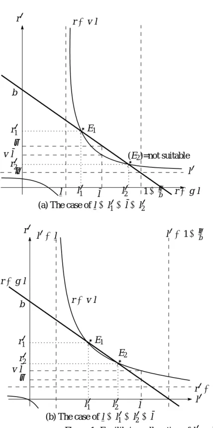
(1+φ˜⁾ρ^,φρ^˜ −ν^¤^. (18) As Figure 1 shows, the intersections of g(l)and v(l)provide the values of r^∗and l^∗ in the steady states. The r^∗value given in (17) must be positive as a necessary condition for a steady state, and therefore l>l must hold, where l≡^{φ ρ}^˜_b and l=l is an asymptote of the function v(l) for the smaller l and r=ν is the asymptote for the larger l. (15) implies that the necessary non-negative condition for r^∗ is r^∗<b, but Figure 1 shows that this is always satisfied. From this discussion, we obtain

b>max[(1+φ˜⁾ρ^, φρ^˜ −ν^, ρ^]^¡⁼^max[(1⁺φ^˜⁾ρ^,φρ^˜ −ν^]^¢ ⁽¹⁹⁾

(11)

To obtain the equilibrium r^∗, we eliminate l using r=g(l) =b(1−l) +ν ^and r=v(l), and thus obtain

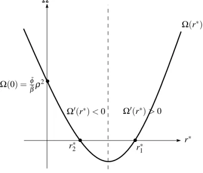
Ω(r^∗)≡r^∗²+r^∗(φρ˜ −b−ν^{) +}φ^˜

β˜ρ²⁼^0. ⁽²⁰⁾ Thus, we transform the existence of the model’s solution(s) into the existence of positive (and less than b) root(s) of the quadratic equation (20). Figure 2 depicts the graph of (20). Using the rule of solutions, we can obtain the analytical r as follows:

r₁^∗= b+ν−φρ˜ ⁺^√^DΩ

2 , and r^∗₂= b+ν−φρ˜ −√ D_Ω

2 , (21)

where D_Ωdenotes the discriminant of the quadratic equation (20) given as follows:

D_Ω≡(φρ˜ −b−ν⁾²−4φρ˜ ²

β˜ ^. ⁽²²⁾

Since Ω(0) = ^φ^˜_˜

βρ²^>^{0, i)} Ω⁰(r^∗=0)<0 and ii) D_Ω >0 are necessary for the existence of positive roots of (20). The condition i) yields positive root(s), if it/they exist(s), and the condition ii) assures the existence of positive root(s), if it/they exist(s).

Condition i) yieldsΩ⁰(r^∗=0) =φρ˜ −b<0, namely b>φρ˜ , which is con- sistent with the positive condition for r^∗ derived from (17). If b<φρ˜ , the equi- librium related to positive long-run growth does not exist. For the case of b>φρ˜ , condition ii) yields

b>φρ˜



1+ 2 q

φ˜β^˜



−ν^. ⁽²³⁾

The case of b<φρ˜ immediately contradicts at least (18). Therefore, the equilibrium related with positive long-run growth cannot be feasible in this case.

Thus, (19) and (23) are necessary conditions that the economy should satisfy in the steady states with a positive growth rate.

Lemma 1 From the existence of a steady state with positive education and pos- itive long-run growth, we have

b>max



(1+φ˜⁾ρ^, φρ^˜ ⁺ν^,



1+ 2 q

φ˜β^˜



φρ˜ −ν



;

(12)

otherwise, the economy is stuck in the steady state related to no education and the 0 long-run growth rate, which is characterized by r^∗=ρ.

We note that the economy with steady state characterized by r^∗=ρ^{; that is,} the one without human capital accumulation, is basically the same as the simple Ramsey model with labor and leisure choice and constant human resources.

The former two conditions in Lemma 1, b>(1+φ˜⁾ρ^{and b}^>φρ^˜ ⁺ν^{, imme-} diately become

φ ^>^max

·ρ

b, ρ

b+ν⁺ρ

¸ .

The last condition in Lemma 1, b >φ˜

·

1+√²_˜

βφ˜

¸

ρ⁺ν yields the following quadratic inequality forp

φ˜^: φ˜⁺q²

β˜ q

φ˜−b+ν ρ ^<^0.

This quadratic inequality and non-negativity ofp

φ˜ gives the following solution:

0<

q φ˜ ^<⁻

1+ r

1+β˜^³^b+_ρ^ν^´ qβ˜ ^.

Since −1+ q

1+β˜^©^(b⁺ν^)/ρ^ª^>0, the inequality has a real solution interval.

We rewrite this condition as

(1>)φ ^> ¹

1+¹_˜

β

³

2+β˜^b+_ρ^ν−2 q

1+β˜^b+_ρ^ν^´^(:=φ^),

where we can easily show φ ^>^{0 using 2}⁺^X ^>²^√¹⁺^{X for X} ^>0. We should note thatφ ∈(0,1), and^∂φ_∂_b<0 and ^∂φ_∂ρ >0. These derivatives imply that the lower limit ofφ is smaller under higher educational efficiency b and a lower subjective discount rateρ^.

From the above discussion, we have the following corollary of Lemma 1:

Corollary From the existence of a steady state with positive education and pos- itive long-run growth, we have

(1>)φ ^>max

·ρ

b, ρ

b+ν⁺ρ^, φ^¸^. (24)

(13)

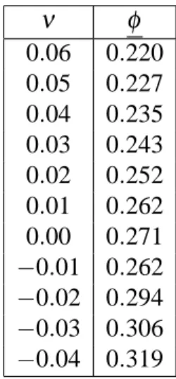
Thus, we obtain the condition of a real root of Ω(r) =0. Here, we provide a numerical discussion. We impose β ⁼0.33.., andν ⁼^{0, where} β is a representative value and ν ⁼0 yields max[ρ^/b,ρ^/(b⁺ν⁺ρ^{)] =}ρ/b, which makes the analysis easier. Table 1 provides the numerical results, where the references for b are as follows: Ladr´on-de-Guevara et al. (1997) use b=0.769, Ladr´on-de- Guevara et al. (1999) use b=0.25, and Mino (2003) uses b=0.15. Thus, we have the result below.

Result 1 Under a plausible specification of b,ρ^{, and}β, the equationΩ(r^∗) =0, which yields the equilibrium interest rate(s), has a (comparatively) broad feasible domain onφ, and a broader domain trend for a lower b and lowerρ^.

Notably, in the preventative case where{β^,^b,ρ^,ν}={0.33,0.25,0.05,0.00}, we obtainφ⁼0.2714.., and the condition (24) in Corollary becomesφ ∈(0.27149,1);

thus, we find that in a broad range ofφ, the Uzawa-Lucas model with labor-leisure choice has feasible steady states.

Next, we check the possibility of multiple steady states. Since (20) is a quadratic equation, the two roots lie on both side of the axis ofΩ(r), whereΩ⁰(·) =0 gives the value of r on the axis. Because (20) has a positive coefficient in the second- order term, the root on the left side of the axis is related by Ω⁰(r^∗) <0, and vice versa. Thus, in this situation, we have two different real number solutions, r₁,r₂,(r₁>r₂), both of which satisfy the following property:

Ω⁰(r) =2r^∗+φρ˜ −b−ν

½ >

<

¾

0 for r=

½ r₁

r₂ . (25)

We next investigate whether r_i(i=1,2)satisfies the feasibility conditions. From bu^∗=ρ ^{in (15), (}E), and the non-negativity of human capital accumulation, we have g^∗_H=b(1−l^∗) +ν−ρ^>0 and l^∗<1−u^∗(=¯l). We also have the condition r^∗=b(1−l^∗)−ν from (13). Uniting these two conditions, we again have the usual positive conditions as r^∗>ρ^{and l}^∗^< ^¯l.

Referring to Figures 1 and 2, we have the following condition:⁵ v¡

¯l¢

<ρ ··· r^∗=r₁

v¡

¯l¢

>ρ ^and Ω⁰(ρ⁾

½ <

>

¾ 0 ···

½ r^∗=r₁, r₂, r^∗=ρ^.

5We should note thatΩ(ρ⁾^>(<)0 corresponds to v(¯l)>(<)ρ^.

(14)

These conditions v¡

¯l¢½ <

>

¾

ρ ^andΩ⁰(ρ⁾

½ <

>

¾

0 become, respectively:

v¡

¯l¢½ <

>

¾

ρ ⇐⇒b

½ >

<

¾ ρ

µ

1+ φ˜ 1−β

¶¡>ρ⁽¹⁺φ^˜⁾^¢ ⁽²⁶⁾

⇐⇒ φ

½ >

<

¾·

1+ µb

ρ⁻¹

¶

(1−β⁾

¸₋1

(≡φ¯^), and

Ω⁰(ρ⁾

½ <

>

¾

0 ⇐⇒ b

½ >

<

¾

ρ⁽²⁺φ^˜⁾−ν ⁽²⁷⁾

⇐⇒ φ

½ >

<

¾ ρ

b+ν−ρ^. Thus, we obtain the following results:⁶

Result 2 We have the following pattern for the steady state(s):

r^∗=r₁ for b>ρ

"

1+ β˜ 1−β

# ,

which yields: 1>φ ^>^max

·ρ

b, ρ

b+ν−ρ^,φ^¯^,φ

¸

(28) r^∗=r₁,r₂ for ρ

"

1+ β˜ 1−β

#

>b>ρ⁽²⁺φ^˜⁾−ν^, which yields: φ¯^>φ ^>^max

·ρ

b, ρ

b+ν−ρ^,φ

¸

. (29)

r^∗=ρ ^for ^b^<ρ⁽²⁺φ^˜⁾−ν^, which yields: max

·ρ

b, ρ

b+ν−ρ^,φ

¸

>φ ^>^0. ⁽³⁰⁾

We note that (29) is possible under the restriction ρ^³¹⁺₁_−β^φ^˜ ^´^>ρ⁽²⁺φ^˜^{) +}ν^, which is

φ ^>β Ã

1−βν˜ ρ

!₋₁

(≡βˆ^). ⁽³¹⁾

6We note that the condition max h _ρ

b+ν+ρ,_b+_ν−ρ^ρ , ..

i

reduces to max h _ρ

b+ν−ρ, ...

i