ESRI Research Note No.33
Measuring Health Care Output
Shigeru Sugihara, Koichi Kawabuchi,
Yasuko Ikemoto, and Ikumi Imamura
July 2017
Economic and Social Research Institute Cabinet Office
Tokyo, Japan
The views expressed in “ESRI Research Note” are those of the authors and not those of the Economic and Social Research Institute, the Cabinet Office, or the Government of Japan. (Contact us: https://form.cao.go.jp/esri/en_opinion-0002.html)
Measuring Health Care Output
1Shigeru Sugihara
2Koichi Kawabuchi
3Yasuko Ikemoto
4Ikumi Imamura
5July 2017
1 This paper was originally presented at the ESRI seminor held on 30 March, 2011. A
change of positions for one of the authors just after the meeting resulted in the delay in its revision.
2 Social and Economic Research Institute, Cabinet Office. 3 Tokyo Medical and Dental University.
4 Social and Economic Research Institute, Cabinet Office. 5 Northern Territories Affairs Administration, Cabinet Office.
Abstract
This paper explores the possibilities of measuring health care output adjusting for quality of care. We explore methods to incorporate quality of health care. First of these adjusts for quality using crude mortality and complication rates. Adjustment of crude rates can be misleading, however, because risk factors change from year to year and chance variation may dominate yearly fluctuations in mortality and complication rates. Hence, second set of indexes incorporates risk-adjusted mortality and complication rates. In controlling for chance variations, we compared three estimation methods which may differ in their ability to control variability of estimates: maximum likelihood, the hierarchical model and autoregressive (AR) restrictions on random effects. Further, to examine how much information is required for reasonable risk adjustment, we compared three risk adjustment models with differing degrees of detailed risk factors. Overall conclusion of the paper is that we do need adjustment of quality of care in the construction of output index of health care. Risk adjustment is also of crucial importance although the choice of method of estimation to control for chance variation may be less crucial. As for the risk factors, the more detailed, the better.
1. Introduction
Measurement of output and deflators in non-market service sectors such as health care is problematic because in these sectors prices are not determined by competitive markets. Often, governments try to correct market mechanisms in these areas through regulation, public insurance, and other measures. Even when governments do not intervene, prices determined in the market do not reflect true consumer preferences thanks to asymmetric information and externalities. Without market prices, proper deflators to use in the calculation of output are hard to obtain.
Recently direct measures of output of non-market service sectors are actively studied and advocated. The Atkinson Review (2005) recommends to measure output directly by counting the number of units for whom services are provided instead of measuring output by aggregating costs of producing the services. In addition, the Atkinson Review (2005) encourages that output is adjusted for the change in quality of services. Eurostat (2001) also recommends direct measurement and quality adjustment. In the United Kingdom, the Office for National Statistics calculates and publishes direct and quality-adjusted output indexes for public sector activities. (Office for National Statistics, 2007, 2008, 2015.) These are based on work done by U.K. researchers (Dawson, et al., 2005). German researchers are investigating how to utilize the DRG system in the direct measurement of health care output (Pierdzioch, 2008). In the United States, pioneering research has been conducted during the 1990s, particularly at the National Bureau of Economic Research, measuring the quality of health care and adjusting for quality change in the calculation of deflators (Cutler and Berndt,eds. 2001). The Bureau of Economic Analysis is now developing a Health Care Satellite Account based on treatments of diseases (Dun, et al., 2015).
A major trend in the practice of National Accounts especially in EU countries is, as is mentioned above, activity-based output index. Activity-based output index measures health care activities such as the number of patients treated or operations performed, and so on. Simple activity-based measure is not appropriate because it is assumed that the more activities are appended, the better. Furthermore, activity-based measure is not unlike input.
A refinement may be to use the DRG system to account for quality of care. This is valid as long as the classification of the DRG system corresponds to quality of care delivered by hospitals. Quality adjustment by the DRG system is not adequate, however. Because the classification typically depends on operations and major procedures, thanks to the choice of treatment on the part of hospitals, not all the patients in the same DRG have
the same severity and, conversely, patients with the same severity do not necessarily belong to the same DRG. Further, output index based on the numbers of patients of DRG classifications could have adverse effects. For example, simply increasing the number of patients by way of “three-minute consultation” will raise the measured output although the quality of care could decline.
Hence, search for more direct methods to adjust for the quality of care are warranted.
In sum, there are two ways to adjust for quality of care. One is activity-based output index, which tries to control quality of care through disaggregation, where disaggregation of health care activities into homogenous activities is assumed to guarantee uniform quality of care within each activity. The other is quality-adjusted output index, which tries to control quality by utilizing explicit measures of quality of care. The goal of these two indexes is the same: adjustment for the quality of care. There is a trade-off between the robustness and refinement of adjustment. Quality adjustment through disaggregation is robust because it does not depend on specific models, while its resultant adjustment is not so complete because the criteria of classification is relatively crude. Quality-adjusted indexe can utilize a rich set of risk factors which affect patients’ outcomes so that its quality adjustment can be refined, while it is not so robust because of its dependency on models used to adjust for risk factors.
This paper first gives examples of construction of activity-based output index covering all diseases. Next, we try to construct output indexes which reflect quality of care. Due to data limitations, we restrict our construction to health care of hospitalized AMI patients. Qualities we consider are mortality and complications. In adjusting for mortality and complications, we first use crude rates, then, we adjust for risk factors of patients.
As for adjustment using crude mortality and complication rates, we compile two indexes. The first one adjusts only for mortality by simply putting utility at zero if a patient dies during hospitalization. In this case, all the patients who are discharged alive are assumed to have the same health utility as the healthy people.
Next, we will try to attach utilities to the case where a patient is discharged alive. We do not have data on the quality of life when a patient survives. We have data on complications, however. We follow Timbie, et al. (2009:Composite Measures paper) in assigning health utilities to individual complications and, then, infer utilities according
as they have the specified complications.
Since risk factors change from year to year, proper risk adjustment is essential. Without controlling for such changes in underlying risk factors, output indexes adjusted for quality of care can be misleading with too much or too little adjustment.
There is no lack of controversies concerning risk adjustment methods. This paper specifically deals with two questions. One is whether it is possible to properly adjust for risk factors despite wild random variation of outcomes in the context of small sample size. The other is how detailed the risk adjustment model should be in view of costly information gathering.
As to the first question, we investigate how statistical methods can cope with chance variation of outcomes by comparing methods differing in their ability to control chance variation.
We consider three estimation methods of a risk adjustment model: the MLE (maximum likelihood estimates), the hierarchical model and AR regression. The second method, the hierarchical model, is especially suitable for controlling chance variation by shrinking individual estimates toward overall mean. The third method imposes restrictions on the rate that quality of care can vary.
As to the second question posed above, we estimated several risk models with various degrees of detailed information. If they imply different mortalities and complications after adjustment, modeling risk factors is of crucial importance.
In sum, we measure health output by adjusting, first, for quality of care and, second, for risk factors. The process and ingredients are summarized as follows.
+ +
Mortality MLE
QOL (Complications) Hierarchical model AR regression
The paper is structured as follows. The second section explains the general framework for output indexes which adjust for quality of care. The third and fourth sections incorporate quality of care into the output indexes, of which the former calculates output indexes adjusted for crude mortality and complications while the latter adjusts risk
factors in measuring the quality of care. The fifth section concludes.
2. A Digression on the Concept of the Quality of Health Care
Output of health care is the improvement of health caused by medical interventions. Therefore, output index should include not only the number of patients but also the improvement of health status attributable to health care. This is what quality-adjusted output index is intended to do.
The concept of the quality of health care can be explained as follows. This exposition is inspired by the discussion in Jacobs, et al. (2006) although much modified. Let the
original health status of a patient at time t be O t
h =0.5. Suppose that when she undergoes
a treatment, her health status will be T t
h =0.7 and that when she does not undergo a
treatment, her health status will be C t
h =0.4. The true quality of care is htT −htC=0.3 while we can observe only O
t T t h
h − =0.2 because we usually do not know the natural history of disease C
t
h .
The Concept of Quality of Health Care Services
Health status T t h O t h C t h Before After intervention intervention
Now suppose that in the next year we have O t h+1=0.5, T t h+1=0.8 and C t h+1=0.4. Namely,
the original health status and the natural history are the same as time t. Then, the quality
of health care at time t+1 is C t T t h
h+1− +1=0.4 while we observe only O t T t h h+1− +1=0.3. However, since O t O t h h+1 = and C t C t h
h+1= , we can calculate the change in the true quality of health care as ( O
t T t h h+1− +1) ( O) t T t h h − − = T t h+1 T t h − . It is not necessarily the case that the original statuses, O
t
h and O
t
h+1, are equal.
Hence, we have to adjust the original statuses in order to compare outcomes, T t
h and
T t
h+1. Risk adjustment just does this. Somewhat formally, we can model the health status
of the treated patient as a function of the original status: ( O)
t t T t f h h = and ) ( 1 1 1 O t t T t f h
h+ = + + . Adjusted health statuses with a common original status, h , are O
) ( O t T t f h h = and 1 1( O) t T t f h
h+ = + . Then, the difference between these two outcomes is the change in quality of health care.
3. Activity-Based Output Indexes
In this section we calculate activity-based indexes with two kinds of units of measure, the ICD and the DPC. These measures cover all diseases. Data used in the construction of activity-based output indexes are taken from public statistics, the Patient Survey and the Analysis and Evaluation of the Effects of the Introduction of the DPC System, which present aggregate data, while the construction in the fifth section of the quality adjusted output index utilizes data collected by authors which consist of data on individual patients. This is because we are not able to classify each patient contained in the latter data set into DPC categories, hence, calculation based on the DPC classification is impossible in the latter data set.
By disaggregating unit of measurement, a homogenous classification of activities may obtain and, hence, quality of output could be accounted for by such detailed
classification. The assumption is that activities directed to a specific classification are of the same quality and that activities directed to different activities are of different quality. Its success depends on, of course, how the classification is done. We will return to this point later.
These indexes are cost-weighted. The quantity of output is weighted by cost assuming that cost is proportional to the marginal social value of output (Castelli, et al., 2007).
∑
∑
⋅ ⋅ = + + i it it i it t i x t c x c x I 1 , 1 ,where x is the quantity of i-th output at time t and it c is unit (average) cost of i-th it
output at time t.
(1) ICD-based unit of measure
Here, activity is defined relative to the ICD diseases. Health care activities devoted to a specific disease are compounded into an activity. It is assumed that quality of health care is the same within a specific disease and different among different diseases. Surely, this assumption is hard to justify. As a reference, however, we calculate output according to this definition. This index is for inpatient services.
Diseases disaggregated to the block level diseases (three digits classification with one alphabet and two numbers) in the ICD system. The data source is the Patient Survey conducted every three years. A finer classification of diseases is available, but we cannot find corresponding costs form the source sited below.
The index is cost-weighted. Cost is the average charge for each ICD disease which is taken from the Survey of Medical Care Activities in Public Health Insurance.
We were able to compile a consistent classification going back from 2008 to 1984. The classification before 1984 is so different that we cannot connect it to the current classification. Further, the 1984 Survey of Medical Care Activities did not include patients covered by the National Health Insurance System. Therefore, we constructed output index from 1987 onward.
The result is shown in Figure 1. Output of inpatient services increased sharply from 1987 to 1990. After that, inpatient output followed a declining trend with especially rapid decrease during the 2000s.
(2) DPC-based unit of measure
The Diagnosis Procedure Combination (DPC) system was introduced in 2003 as a prospective payment system for acute care of patients treated by the Specific Function Hospitals. Thereafter, the DPC system has been expanded to include other eligible hospitals. As of July 2010, the DPC system covers 1,391 hospitals and around 460,000 beds, which account for 50.4% of total beds.
The classification of patients starts with the diagnosis which absorbed resources the most among their diagnoses. Patients are further classified by whether specified operations are performed or not. Then, the final classification is reached according as whether the patient has comorbidities or not.
The DPC system is intended for use in a Prospective Payment System. But it retains characteristics of fee-for-service. For example, payments are per diem, not for the whole hospitalization episode, and the system does not apply to operations and some other costly procedures. Therefore, it provides incentives to reduce LOS as well as incentives to increase operations.
To calculate output index based on the DPC classification the number of patients of each DPC is aggregated with the average length of stay of each DPC as weight. In theory, we should use billing rates as weights. But, since some DPC categories are reimbursed on the fee-for-service basis, billing rates are not available for these categories in the published data. Therefore, we used length of stay as a proxy for cost. It is well documented that the correlation between length of stay and cost is high.
The DPC classification is revised every two years. It is not possible to re-classify patients retrospectively without patient-level data. Every year’s publication of statistics provides data for two years, the current and the previous years, from which we calculated output indexes for two years. Then, we linked these indexes at the overlapping year.
Since the number of hospitals covered by the DPC system is being expanded over time, we cannot simply aggregate the output of hospitals in each year. We restrict the calculation to hospitals which started their participation in 2003, 2004 and 2005. We can obtain data on these hospitals from 2005 through 2009. These hospitals are only a subset of all hospitals and, clearly, early participants in the DPC system have different characteristics from other hospitals. They are large and high-technology-oriented hospitals, in general.
Therefore, the DPC-based output index we constructed is not representative for the entire health care system. However, by comparing the DPC-based index to the raw
number of patients, we can obtain some insight into the extent to which quality adjustment using DPCs as unit of measurement has impact on output index.
Figure 2 shows the growth rates of the output index based on the DPC classification together with the raw number of patients. Overall trend in the output index is similar to the number of patients, but there is a noticeable difference between the two. The difference translates into around 1 % difference in the growth rates in 2006 and 2007.
The DPC classification is meant to be used as a payment system. It is intended to group together diseases with homogenous costs, not disease with homogenous health care activities.
Hence, the classification is heavily dependent on operations performed. This is reasonable from the point of view of the original intention of grouping diseases with homogenous cost. Further, it could be that a specific treatment represents a specific quality of care as in the case of high-technology treatments.
Quality adjustment by the DPC system is not adequate, however.
First, outcomes such as mortality which are expected from specified operations or procedures differ among hospitals and doctors. The same operations and procedures do not always represent the same quality in different hospitals.
Second, the DPC classification is based on the medical procedures selected by health care providers. Inclusion of choice variables into classification criteria may result in problems as statistics. Increase in inappropriate but costly use of medical procedures, such as PCIs for stable coronary patients or low back pain surgeries, will increase the output of health care!
Third, the level of quality of each DPC category is fixed at the beginning. As medical technologies progress, better outcomes are expected to obtain. The measurement based on the DPC system cannot take into account such improvements of outcomes over time.
Fourth, while the DPC system is intended to create homogeneous categories with respect to cost, cost does not necessarily reflect relative levels of quality of DPCs. Costly operations and procedures do not always result in superior outcomes. It is only after we validate the outcomes of individual operations and procedures that we can properly calibrate relative value of each DPC.
Fifth, introduction of output index based on the DPC system could have adverse effects. For example, “three-minute consultation”, for which the Japanese health care
system is notorious, will increase measured output by treating more patients within a given time. “The sooner, the sicker” phenomenon, observed in the United States when the DRG system was introduced, is also a cause for concern. The DPC system imposes a very strong incentive to shorten the length of stay. If shorter length of stay is dictated by economic incentives, there is no guarantee that we have higher quality of care, but again the measured output will rise. Last example to mention is selection bias caused by the gap between the classification and payment systems. Since operations are not included in the DPC payment system, hospitals may be eager to increase the number of operations. Since the DPC classification is dependent on operations, increased operation will result in increase in health care output.
4. General Framework of Quality Adjusted Output Index
We follow Dawson, et al. (2005) and Castelli, et al. (2007) in the construction of quality adjusted output index. Output consists of three components: unit of measurement, quality of care and valuation of the quality. Schematically, we can write:
= × ×
In terms of equation, the above scheme is expressed as follows.
∑ ∑
∑
+∑
+ + = i j jt ijt it i j jt t ij t i x t q x q x I π π 1 , 1 , 1 ,where x is the quantity of i-th output at time t, it q is the quantity of j-th attribute of ijt i-th output at time t and πit is the value of j-th attribute of i-th output at time t.
In this paper, we use data on hospitalized AMI patients, hence, i = AMI. In this case, the above formula simplifies to
∑
∑
+ + + = j jt t j AMI t AMI j jt t j AMI t AMI x t q x q x I π π , , , 1 , , 1 , 1Unit of measurement Quality of care Valuation Output
Unit of measurement is episode of inpatient care. Although cooperation between hospital care and primary care is important factor determining total quality of care, no data are available to evaluate the care process as a whole.
The attributes we will consider include: death, survival with complications and survival without complications. Health utilities we assign are: π=0 for death, π=0.9 for survival without complications and π=0.7 for survival with complications. These numbers will be explained later.
Note that we assigned health utilities to attributes (death and complications). Health utilities are not, strictly speaking, the value of the quality of life in terms of money. In view of the difficulty in evaluating the value of life, however, we avoid assigning monetary valuation of quality of care.
In this section, we construct two indexes adjusting for mortality and complication rates. The first one adjusts only for mortality and the second incorporates quality of life of survivors by adjusting for complications.
First, we adjust only for mortality by simply putting utility at zero if a patient dies during hospitalization. In this case, all the patients who survived are assumed to have the same utility as the healthy people, namely π=1.
Next, we will try to attach utilities to the case where a patient is discharged alive. In the case of output as discharge alive, all the survivors are counted as 1. However, survived patients have different quality of life. Output measure should incorporate this difference, although difficult.
We do not have data on the quality of life when a patient survives. We have data on complications, however. One important factor that affects quality of life is complications during hospitalization. We follow Timbie, et al. (2009) in assigning utilities to individual complications and, then, infer utilities according as patients have the specified complications.
Since risk factors change from year to year, proper risk adjustment is needed. Risk adjustment is done by estimating a logistic regression model to measure the influence of risk factors on mortality.
We compare three methods of estimation of the logistic regression model. The first is maximum likelihood, which is a standard estimation method in statistics. It is pointed out, however, that when estimating random effects as we will do in this paper, their estimates tend to take on extreme values because of small sample variability. Therefore,
some shrinkage is desired by “borrowing” information from other years and shrinking their estimates toward the overall mean. The second approach does just this.
The second estimation method adopts the hierarchical approach to achieve shrinkage. This approach assumes that random effects are exchangeable so that they come from a probability distribution with common mean and variance.
The difference between the first and the second methods is succinctly explained as follows (Spiegelhalter, et al., 2004). Suppose that random variables c ’s come from a t
normal distribution c ~N(0,σ2)
t . MLE corresponds to the case where =∞
2
σ while
the hierarchical model corresponds to the case where 0<σ2 <∞.
The third method imposes autoregressive restrictions on random effects. In this method, a year effects is related to the previous year in the spirit of autoregressive models. Future variability is constrained by the realization of previous year’s random effect and this year’s random errors.
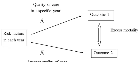
We re-transform the linear predictor in the logistic regression back to the probability scale for individuals. Then, we average across all patients within each year to obtain the predicted outcome. To adjust for case mix differences across years, we follow Timbie, et al. (2009:Cost-Effectiveness paper) who adopted indirect standardization. We estimate counterfactual outcomes for each year assuming underlying quality levels of the entire population while conditioning on each year’s case mix. We take the difference between this expected outcome and the predicted outcome to yield an excess mortality for each year.
Concrete steps of indirect adjustment are the following. Patient mix (distribution of risk factors) is fixed at actual mix in each year for both predicted and expected outcomes. We compare mortality rates of the following two cases for each year. Outcome 1 uses realized quality of care with the relationship between risk factors and outcome being actual one for each year. Outcome 2 uses average quality of care with the hypothetical relationship between risk factors and outcome being estimated by supposing that each year’s quality of care is the same as the total year. Then, excess mortality is calculated as the difference between two outcomes.
Figure 2 Indirect Standardization Quality of care in a specific year βˆ t Excess mortality βt
Average quality of care
5. Adjusting for the Quality of Health Care I: Crude Mortality and Complication (1) Data and Basic statistics
We take as unit of measurement episode of hospitalization of AMI patient. Figure 3 depicts long-term trend of hospitalization of AMI patients in the Patient Survey. The number of AMI patients continued to decline after it peaked in 1990 at a little above 9 thousands. In 2008, the number of hospitalization is a little below 5 thousands, nearly half the level in 1990.
Data were collected on AMI patients in 9 hospitals with a record of hospitalization at some period of time from April 1, 2004 to March 31, 2007 These hospitals had agreed to cooperate in the research for the consecutive years upon approval of in-hospital ethical committee.
We created structured questionnaires for data collection. Questionnaire I asked for detailed clinical information on the patient as well as information on the treatment the patient received. Claim data and physicians profile were collected by Questionnaire II. Questionnaire III collected overall information on AMI treatment at the hospital, such as the annual total number of CABG conducted. A part-time lecturer with physician’s license in Thoracic-Cardiovascular Surgery Section of Tokyo Medical and Dental University stayed throughout the research to fill Questionnaire I from patient medical records including nursing records and discharge summary at each hospital.
Risk factors in each year
Outcome 1
Questionnaire II and III were filled by hospital staffs who were approved of the access to claim data at each hospital.
Sample is restricted to ST-Elevation AMI in the following analyses. This choice is intended to secure homogeneity in the sample as is epitomized by the separate compilation of ACC/AHA guidelines for the management of patients with ST-Elevation myocardial infarction from those for the management of patients with Non-ST-Elevation myocardial infarction.
A data set of patients hospitalized in nine hospitals was constructed. Only the patients hospitalized in hospitals with more than ten STEMI patients in every year are retained in the analysis. Observations are 2631 in total, of which 598 are in 2004, 612 in 2005, 672 in 2006 and 749 in 2007.
Table 1 shows basic statistics of patients for all hospitals. The upper panel contains outcome variables: mortality and complications. The average mortality rate is 10.6% with an upward trend from 2004 to 2007. The average complications rate is 18.4% also with an upward trend. A vast majority of complications is repeat revascularization. Around 5% of survived patients experience complications such as cardiovascular disorder, renal failure and new infarction. The lower panel of Table 1 exhibits basic statistics of risk factors. The Average age is 68.9 years old and a little less than a third patients is female. About a half of patients are in the Killip class 1, a quarter in the class 2 and a little less than 15% in classes 3 and further 14% in the class 4. Occlusion of the left main trunk, left bundle branch block and ventricular fibrillation account for around 4 to 6% of patients, respectively. More than a half of patients are with hypertension and a little less than 40% and a little more than a third are with hyperlipidemia and diabetes mellitus. 8% of patients suffer from heart failure and 10% from renal failure. The share of patients with cancer is 8%.
Table 2 exhibits characteristics of sample hospitals. Three out of nine hospitals are designated as tertiary critical care hospitals and all except one hospitals are designated as teaching hospitals. The average number of beds is 434. Hospitals in the sample are large in general, but the size varies. One hospital holds nearly 1000 beds while two hospitals have less than 200 beds. The average number of AMI patients is 86, but the variation is large. Two hospitals admitted more than 150 AMI patients while two hospitals admitted only around 20. The average number of PCI performed is 297, which is a large number in the Japanese standard. Again, there is a great variation among hospitals. A hospital performed more than 700 PCI while two hospitals performed only a little more than 100 PCI.
Figure 4 shows mortality and complication rates during the sample period. In-hospital mortality increased from 9.2% in 2004 to 12.2% in 2006, then, slightly dropped to 10.8% in 2007. Complication rate is on the upward trend during this period. The complications we use in this paper will be listed below.
(2) Adjusting for crude mortality and complication rates
Two measures are calculated which accounts for quality change. One incorporates only changes in crude mortality. The other adjusts not only for mortality but also for complication rate.
In the case of the first output index which adjusts only for mortality, we put the value of utility π=0 if a patient dies during hospitalization and π=1 if a patient is discharged alive. In this case, no distinction is made between being discharged alive but with complication and being discharged alive without complication.
In the case of the second output index which adjusts not only for mortality but also for complications, the assumed values of utility are as follows (Table 3). We put π=0 if a patient dies during hospitalization. When she survives, we put π =0.9 without complication and π =0.7 with complication. The value of survival without complications is taken from Weintraub, et al. (2008). The value of survival with complications is calculated as follows.
In the adjustment of output for quality of care, complications we use include myocardial infarction, stroke, cardiovascular diseases, renal failure, repeat PCI/emergency CABG and cardiac arrest or shock within 48 hours. Timbie, et al. (2009:Composite Measures paper) provide utility estimates for stroke, renal failure and repeat PCI/emergency CABG. We were unable to find good estimates for the quality of life (QOL) for cardiovascular diseases and cardiac arrest or shock within 48 hours, however. We then proceed in two steps. First, we calculate weighted average of utilities of complications using only stroke, renal failure and repeat PCI/emergency CABG. Weights are the number of patients of each complication in the sample while utility estimates are those of Timbie, et al. (2009:Composite Measures paper). The result isπ=0.77. Second, we adjust the estimate downward a bit toπ=0.7 considering that the remaining complications, cardiovascular diseases and cardiac arrest or shock within 48 hours, appear to be serious ones. The downward adjustment is rather arbitrary, it should be admitted. Caution must be exerted in interpreting the results. In the future, we will improve on the utility estimates of complications to obtain more accurate quality
adjustment.
Figure 5 shows growth rates of output indexes adjusted for crude mortality and complications. The impact of adjustment is substantial, especially in 2006. In 2006, output declined by nearly 4 % without adjustment for mortality while after adjusting for crude mortality, it declined more than 6 %. The difference between growth of output with and without complication adjustment is small. To conclude that adjustment of complications is not essential is premature, though. As is noted above, utility estimates of complications are far from perfect. We should investigate further to answer the question whether complication adjustment is required or not.
It could be very important to adjust for mortality, at least. But this conclusion can be premature again because change in mortality reflects not only underlying change in the quality of care, but also change in risk factors and chance variation of mortality. The next section will deal with this problem.
6. Adjusting for the Quality of Health Care II: Risk Adjustment (1) Methods
We follow the method taken by Timbie, et al. (2008:Cost-Effectiveness paper). We created a measure of disease severity, severity index, for each patient. A logistic regression was used to model the effect of demographic and clinical risk factors of in-hospital mortality. Risk factors are selected by checking statistical significance and signs of estimated coefficients. Risk factors include age, female,Killip classes 2, 3 and 4, occlusion of the left main trunk, left bundle branch block (LBBB), ventricular fibrillation, hypertension, hyperlipidemia, diabetes mellitus, heart failure, history of myocardial Infarction, history of PCI, history of CABG, cancer, bleeding tendency, renal failure , cerebrovascular diseases, aneurysm and Chronic Obstructive Pulmonary Disease (COPD). The adopted risk factors are not far from those proposed in Krumholz, et al. (2006: Administrative Claims Model paper) on which Timbie, et al. (2008) base their construction of severity variable. Estimation result is shown in Appendix Table A1. Severity index is estimated as a linear predictor using the coefficients from the estimated logistic regression:
∑
= ⋅ = P p itp p it x severity 1 ˆ β ,where x denotes p-th covariate of i-th patient at time t. Age is centered at the sample itp
mean.
(i) MLE
To adjust for risk factors, we estimated logistic regression models with outcomes as
dependent variables. The outcome variable, yit, takes the value one if a patient i in time t dies and zero if she survives. In this subsection, we estimated this model by the maximum likelihood method.
logit[p(yit =1|xit)]=αt +βt⋅xit
where x is severity index. Then we re-transform the linear predictor into the original it
probability scale: ) ( ) exp( 1 ) exp( ) | 1 ( t t it it t t it t t it it x x x x y p ≡Λ + ⋅ ⋅ + + ⋅ + = = α β β α β α
The resulting estimates are used to calculate excess mortality by way of indirect standardization. As is explained above, indirect standardization compares mortality rates of the following two cases for each year: Outcome 1 which uses realized quality of care and Outcome 2 which uses average quality of care.
Outcome 1 utilizes actual relationship between risk factors and mortality for each year so that parameters are estimated using the sample of each year separately. Parameters, αt and βt, depend on time t.
] 0 [ 1 + ⋅ + > = t t it it it x u y α β
Once we obtain estimates, αˆ andt βˆt, we re-transform the linear predictor into the original probability scale:
) ˆ ˆ ( ) | 1 ( ˆ yit xit t t xit p = =Λα +β ⋅
Then, we average individual probabilities of death for each year: t = 2004, 2005, 2006 and 2007. ) ˆ ˆ ( 1 ˆ 1 it t t n i t t x n D t ⋅ + Λ =
∑
= β αThen survival rate is Eˆt =1−Dˆt.
Outcome 2 sets up a hypothetical relationship between risk factors and mortality for each year by supposing that each year’s quality of care is the same as the average year. Parameters are estimated using the sample from all years so that parameters, α and β,
do not depend on t: common parameters for all years.
] 0 [ 1 + ⋅ + > = it it it x u y α β
With the estimates, α and β , we re-transform the linear predictor into the original probability scale: ) ( ) | 1 (yit xit xit p = =Λ α +β ⋅
Again, we average individual probabilities of death for each year: t = 2004, 2005, 2006 and 2007. ) ( 1 1 it n i t t x n D t ⋅ + Λ =
∑
= β αThen survival rate is Et = 1−Dt.
(ii) Hierarchical Model
Logistic regression model is estimated with random intercept, αt, for each year and random coefficient, βt, for each year.
] 0 [ 1 + ⋅ + > = t t it it it x u y α β
Prior specifications are as follows. Two random coefficients are assumed to follow
bivariate normal with a mean vector, µ , and a precision matrix Σ : −1 c ~N(µ,Σ−1)
t with ≡ t t t c β α
. The random effect, c , for each year comes from the same normal t
distribution so that shrinkage toward the overall mean, µ , is expected.
µ is assumed to follow a normal distribution with mean 0 and variance 100: ) 100 , 0 ( ~ N
µ . The choice of the variance of 100 is intended to represent a diffuse prior. Gelman and Hill (2007) give a thoughtful discussion on the appropriateness of this value in the context of the logistic models or log-transformed regressors. They argue that in logistic and logarithmic regressions, typical changes in outcomes are on the scale of 0.1 or 1, but not 10 or 100, so that one would not expect to see coefficients much higher than 10 in absolute values as long as the regressors are also on a reasonable scale. Their choice of the value of variance is 2
100 (standard deviation of 100), which states, roughly, that we expect the coefficient to be in the range (-100, 100). Our choice 10 2 implies that the expected range is (-10, 10). We believe that this range is wide enough so that the prior distribution is providing little information in the inference. In fact, mean estimates of µ obtained below are (-3.77, 1.03), which are well in the range (-10, 10).
The precision matrix is assumed to follow Wishart distribution with scale matrix Ω and 2 degrees of freedom: Σ−1 ~Wishart(Ω,2). The choice of the 2 degrees of freedom is intended to represent diffuse prior. Ωis, in turn, specified as I2.
The model was estimated with Markov chain Monte Carlo methods using WinBUGS software. To check the convergence, three parallel chains were run to calculate the Gelman-Rubin statistic. A burn-in of 10,000 iterations for each chain was allowed for the model to converge. Additional 20,000 samples for each chain were drawn from the joint posterior distribution for the estimation of all model parameters.
(iii) AR Restrictions
Logistic regression model is estimated with random intercept, αt, for each year and random coefficient, βt, for each year. AR restrictions are imposed on the movement of random effects over time.
] 0 [ 1 + ⋅ + > = t t it it it x u y α β t t t t =γ ⋅α−1+v α α t t t t =γ ⋅β−1+w β β
To calculate the effect on mortality of random effect for each year, we re-transform the linear predictor into the original probability scale in the same way as MLE.
The model was estimated with Markov chain Monte Carlo methods using WinBUGS software. The number of chains, check of convergence, burn-in and samples for estimation are the same as the hierarchical model.
Prior specifications are also similar. Random intercept for each year, αt, is assumed to follow a normal distribution with mean µαt and variance, 2 12
t t α α σ σ ≡ : ) , ( ~ t 2t t N µα σα
α . µαt is assumed to follow a normal distribution with mean 0 and variance 100: µαt ~ N(0,100).
A uniform prior on the standard deviation, σαt, is adopted: σαt ~ Uniform(0,100) The coefficient, γαt, on AR relations between αt’s and other parameters are assumed to follow normal distributions with mean zero and variance 100: γαt ~ N(0,100), etc.
Similar priors are specified for βt and γβt.
(2) Results
Estimation results for the cases of MLE, hierarchical priors and AR restrictions are shown in Appendix Tables A2, A3 and A4 for mortality and Table A6, A7 and A8 for complications. Pooled estimations are in Tables A5 for mortality and A9 for complication.
Crude and adjusted rates differ more than one percentage point in 2004 and 2006. Hence, risk adjustment exerts significant influences on the mortality. The difference among different risk-adjustment methods is small. One possibility is that the sample includes several hundreds of patients for each year so that chance variations are well controlled by even the MLE.
Figure 7 contrasts crude complication rates with risk-adjusted complication rates. The complication rates estimated with MLEs are not greatly different from the crude rates. In the cases of hierarchical prior and AR restriction, crude and adjusted rates differ significantly. The differences between the case of MLE and the cases of hierarchical prior and AR restriction are relatively large. Recognizing that our adjustment for complications is rudimentary, we may suspect that the hierarchical model may be required in the case of noisy data.
Figures 8, 9 and 10 show growth rates of output indexes with risk adjustment by MLE, hierarchical priors and AR restrictions. Overall behavior is the same as the case of adjustment by crude rates shown in Figure 6. However, the magnitude of adjustment is much smaller than the latter case.
To see this more clearly, Figures 11 and 12 superimpose growth rates by various adjustment methods. In 2006, for example, the magnitude of adjustment with risk adjustment is around half the magnitude of the case by crude rates.
This indicates that quality adjustment by crude rates is too much. Change in the mortality and complication rates include not only true change in the quality of care but also change in risk factors. Therefore, not all the changes in the output index adjusting for quality by crude rates does not represent changes in quality-adjusted output.
(3) How much is enough? – Comparing Various Severity Indexes
A remaining question is: do we need detailed risk adjustment or is it sufficient to adjust for only basic demographic factors? To examine this question, we created two additional severity indexes which involve different degrees of risk adjustment. First one, denoted as severity 2, includes only age and female. The second one, denoted as severity 3 includes, in addition to age and female, Killip classes, ventricular fibrillation and renal failure.
Excess mortalities are calculated using these additional severity indexes. Here, excess mortality means deviation from the four-year average. The results are shown in Figure 13. The mortality adjusted with severity 2 is not very different from the crude mortality. The mortality adjusted with severity 3 is half way between the crude mortality
and the mortality with baseline severity index.
Therefore, the extent of risk adjustment exerts significant impact on the estimates of adjusted mortality, and hence on the output index.
7. Conclusion
In this paper we investigated the question: how to measure output of health care. We explored methods to incorporate quality of health care.
First of these adjusts for crude mortality and complication rates. Adjustment of crude rates can be misleading, however, because risk factors change from year to year and chance variation may dominate yearly fluctuations in mortality and complication rates.
Hence, second set of indexes incorporates risk-adjusted mortality and complication rates. In controlling for chance variations, we compared three estimation methods: maximum likelihood, the hierarchical model and autoregressive (AR) restrictions on random effects.
Further, to examine how much information is required for reasonable risk adjustment, we compared three risk adjustment models with differing degrees of detailed risk factors.
Overall conclusion of the paper is that we do need adjustment of quality of care in the construction of output index of health care. Mortality adjustment has much larger impact than complication adjustment. However, our adjustment of complications is far from perfect. It is very important to improve on adjustment of complications in the future research.
Risk adjustment is also of crucial importance although the choice of method of estimation to control for chance variation may be less crucial. This is especially true in the case of mortality adjustment. One possibility is that the sample includes several hundreds of patients for each year so that chance variations are well controlled by even the MLE. In the case of complication adjustment, however, the differences between the results of MLE and the hierarchical model are relatively large. Recognizing that our adjustment for complications is rudimentary, we may suspect that the hierarchical model may be effective in the case of noisy data with measurement error.
As for the risk factors included in risk adjustment, the more detailed, the better.
because of data limitation. Methods in this paper (or improved ones) to incorporate quality of care in output index can be applied to health care in general.
The fundamental barrier to the measurement of health care output is data limitation. It is imperative to enrich our data environment by routinely collecting detailed data on risk factors and outcomes, especially quality of life.
It would be best to directly measure health utility by way of established instruments such as EQ-D5 or SF-36, but such direct measurement may be impractical. Stewart, et al. (2005) proposed to relate data on symptoms and impairments to health utility in order to monitor population health. If we collect data on symptoms and impairments of patients, we can infer health utility of individual patients by assigning health utilities to complications.
References
Abraham, Katharine G., and Christopher Mackie, eds. (2005) Beyond the Mark et: Designing
Nonmark et Accounts for the United States. National Academies Panel on Conceptual, Measurement
and Other Statistical Issues in Developing Cost-of-Liv ing Indexes. Washington, DC: The National Academies Press for the National Research Council.
Aizcorbe, Ana, Bonnie Retus and Shelly Smith. (2007) Toward a Health Care Satellite Account.
Survey of Current Business, May 2007.
Atkinson, Tony (2005) Atk inson Review: Final Report. Measurement of Government Output and
Productivity for the National Accounts.
Aiguilar, Oma r, and Mike West. (1999) Analysis of Hospital Quality Monitors Using Hierarchical Time Series Models. In C. Gatsonis, et al., eds., Case Studies in Bayesian Statistics, vol.9, pp.287-302.
Berndt, Ernst R., Susan H. Busch and Richard G. Frank. (2001) Treatment Price Indexes for Acute Phase Major Depression. In David Cutler and Ernst Berndt, eds. Medical Care Output and
Productivity, University of Chicago Press, pp.463-505.
Berndt, Ernst, David Cutler, Richard Frank, Zvi Griliches, Joseph Newhouse and Jack Triplett. (2001) Price Indexes for Medical Care Goods and Service: An Overview of Measurement Issues. In David Cutler and Ernst Berndt, eds. Medical Care Output and Productivity, University of Chicago Press, pp.141-198.
Birkmeyer JD, Siewers AE, Finlayson EVA, Stukel TA, Lucas FL, Batista I, Welch HG, Wennberg DE Birkmeyer JD, Siewers AE, Finlayson EVA, Stukel TA, Lucas FL, Batista I, Welch HG, Wennberg DE. (2002) Hospital Volu me and Surgical Mortality in the United States. New England
Journal of Medicine 346:1128-1137.
Birkmeyer JD, Stukel TA, Siewe rs AE, Goodney PP, Wennberg DE, Lucas FL. (2003) Surgeon Vo lume and Operative Mortality in the United States. New England Journal of Medicine 349:2117-2127.
Spertus JA, Krumholz HM. Hospital quality for acute myocardial infarction: correlat ion among process measures and relationship with short-term mortality. Journal of the American Medical
Association 2006; 296:72–78.
Bronskill, Susan, Sharon-Lise Normand, Mary Landrum and Robert Rosenheck. (2002) Longitudinal Profiles of Health Care Providers. Statistics in Medicine 21: 1067-1088.
Burgess, James, Cindy Christiansen, Sarah Michalak and Ca rl Morris. (2003) Medical profiling: improving standards and risk adjustments using hierarchical models. Journal of Health Economics,
19(3): 291-309.
Carey, K., Burgess, J.: On measuring the hospital cost/quality trade-off. Health Economics 8, 509–520 (1999)
Castelli, Adriana, Diane Dawson, Hugh Gravelle and Andrew Street. (2007) Improving the Measurement of Health System Output Growth. Health Economics 16: 1091-1107.
Castelli, Adriana, Mauro Laudicella and Andrew Street. (2008) Measuring NHS Output Growth
CHE Research Paper 43, Centre for Health Economics, University of York.
Castelli A, Laudicella M, Street A, Ward P. Getting out what we put in: productivity of the English NHS. Health Economics, Policy and Law; Forthcoming.
Cle ment, J.P., Va ld manis, V.G., Ba zzoli, G.J., Zhao, M., Chukma itov, A.: Is more better? An analysis of hospital outcomes and efficiency with a DEA model of output congestion. Health Care
Management Science 11, 67–77 (2008)
Cutler, David and Ernst Berndt, eds. (2001) Medical Care Output and Productivity, University of Chicago Press.
Cutler, David and Mark McCle llan. (2001) Is Technological Change in Medicine Worth IT? Health
Affairs 20(5): 11-29.
Cutler, David, Mark McClellan, Joseph Newhouse and Dahlia Remler. (1998) Are Medical Prices Declin ing? Evidence from Heart Attack Treatment. Quarterly Journal of Economics 113(4): 991-1024.
Cutler, David, Mark McCle llan, and Joseph P. Newhouse. (1999) The Costs and Benefits of Intensive Treatment for Ca rdiovascular Disease. In Jack Trip lett, ed., Measuring the Prices of
Medical Treatments, Washington, D.C.: The Brookings Institution, 34-71.
Cutler, David M., and Elizabeth Richardson. (1999) Your Money and Your Life: The Value of Health and What Affects It. In Alan M. Garber ed., Frontiers in Health Policy Research, Vol. 2, Cambridge, MA: MIT Press, pp. 99-132.
Cutler, David, Allison Rosen and Sandeep Vijan. (2006) The Va lue of Medical Spending in the U.S., 1960-2000. New England Journal of Medicine 355(9): 920-927.
Daniels MJ, Gatsonis C. (1999) Hierarchica l generalized linear models in the analysis of variations in health care utilization. Journal of the American Statistical Association 94(445):29–42.
Daniels MJ, Normand SLT. (2006) Longitudinal profiling of health care units based on continuous and discrete patient outcomes. Biostatistics 7(1):1–15.
Dawson D, Gravelle H, O'Mahony M, Street A, Weale M, Castelli A, Jacobs R, Kind P, Loveridge P, Martin S, Stevens P and Stokes L. Developing new approaches to measuring NHS outputs and productivity. Centre for Health Economics, University of York; CHE Research Paper 6; 2005.
Draper, David, and Mark Gittoes. (2004) Statistical analysis of performance indicators in UK higher education. Journal of the Royal Statististical Society series A, 167, Part3, pp. 449–474.
Duan, N. (1983) Smearing estimates. Journal of the American Statistical Association 78: 605-610.
Dun, Abe, Lindsey Rittmueller and Bryn Whitemire. (2015) Introducing the New BEA Hea lth Care Satellite Account. Survey of Current Business, January 2015, pp.1-21.
Eurostat (2001) Handbook of Price and Volume Measures in National Accounts.
Evans, David, Ajay Tandon, Christopher Murray and Jeremy Lauer. (2000) The Comparative Efficiency of National Health Systems in Producing Health: An Analysis of 191 Countries. GPE Discussion Paper, No.29, World Health Organization.
Fisher, Elliott S., David E. Wennberg, Thérèse A. Stukel, Danie l J. Gottlieb, F. L. Lucas, and Étoile L. Pinder. (2003) The Implications of Regional Variat ions in Medicare Spending. Part 1: The Content, Quality, and Accessibility of Care. Part 1, Annals of Internal Medicine, Feb 2003; 138: 273 - 287. Part 2, Ann Intern Med, Feb 2003; 138: 288 - 298.
Ford, Earl S., Umed A. Ajani, Janet B. Croft, et al. (2007) Explaining the Decrease in U.S. Deaths from Coronary Disease, 1980–2000. New England Journal of Medicine 356: 2388-2399.
Fukui, Tadashi and Yasushi Iwamoto. (2004) Medical Spending and the Health Outcome of the Japanese Population. A paper for ESRI International Joint Research Project.
Garber, Alan, and Jonathan Skinner. (2008) Is American Health Care Uniquely Inefficient? Journal
of Economic Perspectives 22(4): 27-50.
Gelman, Andrew, and Jennifer Hill. (2007) Data Analysis Using Regression and
Multilevel/Hierarchical Models. Cambridge University Press.
Go ldstein, Harvey, and David Spiegelhalter. (1996) League Tables and Their Limitations: Statistical Issues in Co mparisons of Institutional Performance. Journal of the Royal Statistical Society Series A 159: 385-443.
Granger CB, Steg PG, Peterson E, et a l. (2005) Medication performance measures and mortality following acute coronary syndromes. American Journal of Medicine 118:858-865.
Greene, Willia m. (2005) Reconsidering Heterogeneity in Panel Data estimators of the Stochastic Frontier Model. Journal of Econometrics 126: 269-303.
Hvenegaard A, Nie lsen Arendt J, Street A, Gyrd-Hansen D. (2010) Exp loring the relationship between costs and quality: Does the joint evaluation of costs and quality alter the ranking of Danish hospital departments? European Journal of Health Economics
Hannan EL, O’Donnell JF, Kilburn H Jr, Bernard HR, Yazici A. (1989) Investigation of the relationship between volume and mortality for surgical procedures performed in New York State hospitals. Journal of the American Medical Association 262:503-510.
Halm, Ethan, Clare Lee and Mark Chassin. (2000) How Is Volume Related to Quality in Health Care? A Systematic Review of the Research Literature. In Interpreting the Volume-Outcome
Relationship in the Context of Health Care Quality. Maria Hewitt for the Committee on the Quality of Health Care in America and the National Cancer Policy Board. Wachington DC: Institute of Medicine, National Academy Press.
Hollingworth, Bruce. (2003) Non-Parametric and Parametric Applications Measuring Efficiency in Health Care. Health Care Management Science 6: 203–218.
Hollingsworth, B.: The measurement of efficiency and productivity of health care delivery. Health
Economics 17, 1107–1128 (2008)
Jacobs R, Smith PC, Street A. Measuring Efficiency in Health Care: Analytic Techniques and Health
Policy. Cambridge University Press, 2006.
Kawabuchi, Koichi, and Shigeru Sugihara. (2006) Vo lume -Outcome Re lationship in Japan: the Case of Percutaneous Transluminal Coronary Angioplasty (PTCA) Volu me on Mortality of Acute Myocardial Infarction (AMI) Patients. In David Wise and Naohiro Yashiro, eds., Health Care Issues
in the United States and Japan (National Bureau of Economic Research Conference Report),
University of Chicago Press, 2006, pp.113-145.
Kru mholz HM, Wang Y, Mattera JA, et al. (2006) An administrative claims model suitable for profiling hospital performance based upon 30-day mortality rates among patients with an acute myocardial infarction. Circulation 113:1683-1692.
Landrum MB, Bronskill SE, Normand S-LT. (2000) Analytic methods for constructing cross-sectional profiles of health care providers. Health Services and Outcomes Research
Methodology 1(1):23–47.
Landrum, Mary, Sharon-Lise Normand and Robert Rosenheck. (2003) Selection of Re lated Multivariate Means: Monitoring Psychiatric Care in the Department of Veterans Affairs. Journal of
the American Statistical Association 98: 7-16.
Luciano, Mariagrazia. (2006) Measurement of non-market output in education. Paper prepared for the joint OECD/ONS/Government of Norway workshop ”Measurement of non-market output in education and health” London, Brunei Gallery, October 3 – 5, 2006.
Harvey Goldstein, eds., Multilevel Modelling of Health Statistics. John Wiley & Sons, pp.127-142.
Mark B. Mc Cle llan. (1997) Hospital Reimbursement Incentives: An Empirical Analysis. Journal of
Economics and Management Strategy, Vol. 6 no. 1, page(s) 91-128.
McClellan, Mark, Barbara J. McNeil, and Joseph P. Newhouse. (1994) Does More Intensive Treatment of Acute Myocardial Infarction Reduce Mortality? Journal of the American Medical
Association, 272(11): 859-866.
McClellan, Mark and Douglas Staiger. (1999) The Quality of Health Care Providers. NBER Working Paper No.7327.
McClellan, Mark and Douglas Staiger. (2000) Comparing the Quality of Hea lth Care Providers.In Alan Garber (ed.) Frontiers in Health Policy Research, Volu me 3. 2000, The MIT Press, Ca mbridge MA, pp. 113-136.
McKay, N.L., De ily, M.E. (2008) Cost inefficiency and hospital health outcomes. Health Economics 17, 833–848.
Morey, R.C., Fine, D.J., Loree, S.W., Retzlaff-Roberts, D.L., Tsubakitani, S. (1992) The trade-off between hospital cost and quality of care. An exploratory empirical analysis. Medical Care 30, 677–698.
Murphy, Kevin M. and Robert H. Topel (2006) “The Value of Health and Longevity,” Journal of
Political Economy, Vol. 114, pp. 871–904.
Murray, Christophe, and David Evans, eds. (2003) Health Systems Performance Assessment: Debates, Methods and Empiricism. World Health Organization.
National Research Council. (2008) Strategies for a BEA Satellite Health Care Account. Summary of a Workshop, National Academies Press.
Nordhaus, William D. 2003. “The Health of Nations: The Contribution of Improved Health to Living Standards.” In Measuring the Gains from Medical Research: An Economic Approach, edited by Kevin M. Murphy and Robert H. Topel. Chicago: Univ. Chicago Press.
Normand SLT, Glic kman ME, Gatsonis CA. (1997) Statistical methods for profiling providers of medica l care : issues and applications. Journal of the American Statistical Association 92(439):803–814.
OECD (2000) A System of Health Accounts.
O’Hagan A, Stevens JW. (2001) A fra me work for cost-effectiveness analysis from c lin ical tria l data.
Health Economics 10:303–315.
Orosz, Eva. (2005) The OECD System of Health Accounts and the US National Hea lth Accounts: Improving Connections through Shared Expe riences. Paper Prepared for the conference on “Adapting National Health Expenditure Accounting to a Changing Health Care environment”. Centers for Medicare and Medicaid Services, 21-22 April 2005.
Orosz, Eva, and David Morgan. (2004) SHA-Based Bational Health Accounts in Thirteen OECD Countries: A Comparative Analysis. OECD Health Working Papers No.16.
Peterson ED, Rose MT, Mulgund J, et al. (2006) Association between hospital process performance and outcomes among patients with acute coronary syndrome. JAMA 295:1912-1920.
Rosen, Allison, and David Cutler. (2007) Measuring Medical Care Productivity: A Proposal for U.S. National Health Accounts. Survey of Current Business, June 2007.
Skinner, Jonathan, Elliott Fisher and John Wennberg. (2005) The Effic iency of Medicare. In David Wise, ed., Analyses in the Economics of Aging, pp. 129 – 160.
Skinner, Jonathan, and Douglas Staiger. (2009) Technology Diffusion and Productivity Growth in Health Care. NBER Working Paper No. 14865.
Skinner, Jonathan , Douglas Staiger and Elliott Fisher. (2006) Is Technological Change in Medicine Always Worth It? The Case of Acute Myocardial Infarction. Health Affairs, 25(2): w34-w47.
Smith, Peter, and Andrew Street. (2006) Analysis of Secondary School Efficiency: Final Report. Research Report No.788, Department of Education and Skill, UK.
in the Public Sector, CHE Research Paper 16, Centre for Health Economics, University of York.
Spertus, John A., Martha J. Radford, Nathan R. Every, et al. (2003) Challenges and Opportunities in Quantifying the Quality of Care for Acute Myocardial Infarction. Circulation, vol.107, pp.1681-1691.
Spiegelhalter, David, Abrams, Keith R., Myles, Jonathan P. (2004) Bayesian Approaches to Clinical
Trials and Health Care. John Wiley & Sons.
Spiegelhalter DJ, Tho mas A, Best NG, Gilks WR. (1996) BUGS: Bayesian Inference Using Gibbs
Sampling.
Staiger, D. O., J. B. Dimick, O. Baser, Z. Fan, and J. D. Birkmeyer. (2009) Empirica lly derived composite measures of surgical performance. Medical Care 47(2):226-233.
Street A, Hakkinen U. Health system productivity and efficiency. In: Smith PC, Mossialos E, Leatherman S, Papanicolas IN, editors. Performance measurement for health system improvement: experiences, challenges and prospects: World Health Organization; 2009.
Street A, Scheller-Kre insen D, Geissler A, Busse R (2010): Determinants of hospital costs and performance variation: Methods, models and variables for the EuroDRG pro ject. Working Papers in Health Policy and Management Vol. 3 May 2010, Berlin: Universitätsverlag der TU Berlin.
Street A, Dawson D (2002) Costing Hospital Activity: the Experience with Healthcare Resources Groups in England. European Journal of Health Economics 3: 3-9.
Stewart, Susan, Rebecca Woodward, Allison Rosen and David Cutler. (2007) A Proposal for Monitoring Symptoms, Impairments and Health Ratings. NBER Working Paper No.11358.
Justin Timbie , Joseph Newhouse, Meredith Rosenthal, Sharon-Lise Normand. (2008) A Cost-Effectiveness Frame work for Profiling the Value of Hospital Care. Medical Decision Making 28: 419-434.
Justin W. Timbie , David M. Shahian, Joseph P. Newhouse, Meredith B. Rosenthal and Sharon-Lise T. Normand. (2009) Co mposite measures for hospital quality using quality-adjusted life years. Statistics
Justin W. Timb ie and Sharon-Lise T. Normand. (2008) A comparison of methods for combining quality and efficiency performance measures: Profiling the value of hospital care
following acute myocardial infarction. Statistics in Medicine 27:1351–1370
Triplett, Jack. (2000) What’s Different about Health? In David Cutler and Ernst Berndt, eds. Medical
Care Output and Productivity, University of Chicago Press, pp.15-94.
UK Department of Health. (2005) Healthcare Output and Productivity: Accounting for Quality
Change.
UK Office for National Statistics. (2007) The ONS Productivity Handbook : A Statistical Overview
and Guide.
UK Office for National Statistics. (2008) Sources and Methods for Public Service Productivity:
Health.
UK Office for National Statistics. (2015) Public Service Productivity Estimates: Healthcare 2013.
Viscusi W, Aldy J. (2003) The value of a statistical life: a c ritica l review of ma rket estimates 504 throughout the world. Journal of Risk and Uncertainty, vol. 27(1), pages 5-76.
Weintraub, Willia m, Willia m Boden, Zugini Zhang, et al. (2008) Cost-Effectiveness of Percutaneous Coronary Intervention in Optimally Treated Stable Coronary Patients. Circulation Cardiovascular
Quality and Outcomes 1: 12-20.
Gappei 0.046 0.042 0.024 0.053 0.061 New infarction 0.006 0.007 0.005 0.007 0.004 Cardiovascular disorder 0.033 0.026 0.013 0.044 0.045 Renal failure 0.010 0.011 0.007 0.005 0.015 Stroke 0.001 0.004 0.000 0.000 0.001 Repeat revascularization 0.183 0.176 0.169 0.192 0.192 Repeat PCI 0.164 0.153 0.142 0.181 0.177 Emergency CABG 0.022 0.029 0.032 0.010 0.016 Change within 48 hours 0.002 0.002 0.005 0.000 0.000 Cardiac arrest 0.000 0.000 0.000 0.000 0.000 Shock 0.002 0.002 0.005 0.000 0.000 Note: Figures for complications are based on survivors only.
Risk fctors Total 2004 2005 2006 2007
Age 68.9 68.9 68.8 69.0 69.0 Female 0.296 0.298 0.289 0.275 0.320 Killip1 0.482 0.527 0.430 0.510 0.462 Killip2 0.237 0.199 0.288 0.211 0.248 Killip3 0.147 0.124 0.119 0.153 0.183 Killip4 0.135 0.151 0.163 0.125 0.107 Left main trunk occluded 0.051 0.042 0.052 0.058 0.052 LBBB 0.067 0.057 0.072 0.061 0.075 Ventricular fibrillation 0.044 0.030 0.031 0.064 0.048 Hypertension 0.539 0.587 0.565 0.487 0.525 Hyperlipidemia 0.375 0.375 0.355 0.360 0.405 Diabetes mellitus 0.348 0.370 0.364 0.351 0.314 Heart failure 0.078 0.100 0.078 0.063 0.075 History of myocardial infarction0.108 0.100 0.127 0.112 0.093 History of PCI 0.095 0.107 0.101 0.095 0.081 History of CABG 0.015 0.007 0.018 0.022 0.013 Cancer 0.076 0.060 0.056 0.098 0.087 Bleeding 0.019 0.020 0.029 0.015 0.015 Renal failure 0.102 0.119 0.090 0.116 0.085
The number of hospital beds
Total hospital
patients AMI patients
The number of PCI (Average/year) (Average/year) (Average/year) (Average/year)
(2006-2009) (2006-2009) (2006-2009) (2006-2009) 1 ◎ ○ 956 304,183 164 483 2 ○ ○ 524 89,224 69 103 3 ○ ○ 322 7,839 19 109 4 ○ ○ 530 1,601 81 299 5 ○ ○ 202 72,410 186 712 6 ◎ ○ 592 187,739 89 253 7 ◎ ○ 469 159,961 93 185 8 ○ - 151 27,275 22 163 9 ○ ○ 165 3,198 50 367 434 94,826 86 297
1) ◎: Tertiary Emergency Care, ○ : Secondary Emergency Care
"Tertiary Emergency Care"-provide patients with high-acuity conditions who require admission to the intensive care or emergency surgery. "Secondary Emergency Care"-provide patients with moderate-acuity conditions who require admission to a general inpatient bed.
The level of designated Emergency Care 1) The status of clinical resident training hospital hospit al I D Average of 9 hospitals