University of Siegen, Kobe University and Muroran Institute of Technology at TRECVID 2013 Multimedia Event Detection

University of Siegen, Kobe University and Muroran Institute of Technology at TRECVID 2013 Multimedia Event Detection

Kimiaki Shirahama, Chen Li and Marcin Grzegorzek Research Group for Pattern Recognition, University of Siegen

Hoelderlinstrasse 3, 57076 Siegen, Germany

{kimiaki.shirahama,chen.li,marcin.grzegorzek}@uni-siegen.de Kuniaki Uehara

Graduate School of System Informatics, Kobe University 1-1, Rokkodai, Nada, Kobe 657-8501 Japan

[email protected]

Abstract

This paper presents our method developed for TRECVID 2013 Multimedia Event Detection task. The following two problems are mainly addressed: The first is weakly supervised setting where training videos contain many shots irrelevant to a target event. The other is the diversity of visual appearances, meaning that shots relevant to the event are characterised by significantly different visual appearances. To overcome these prob- lems, Hidden Conditional Random Fields (HCRFs) are used where the event is detected by assigning shots in a video to hidden states, each of which represents the compatibility between a feature combination and the event label. Although our submitted run SiegenKobe- Muro MED13 VisualSys PROGAll PS 100Ex 6 on the progress search set was ranked at the low position (MAP of 4.1%), preliminary experiments on MED Test Background set show the effectiveness and potential of our method.

1. Introduction

TREC Video Retrieval Evaluation (TRECVID) is an an- nual worldwide competition where large-scale benchmark video data are used to evaluate methods developed all over the world [13]. Through this competition, TRECVID aims to promote progress in video analysis and retrieval. At TRECVID 2013 [8], we participated in the Multimedia Event Detection (MED) task to identify videos where a cer- tain event occurs. Our method developed for this is pre- sented in this paper.

The MED task can be considered as a binary classifi-

cation problem to construct a classifier that distinguishes videos showing an event from the other videos. The event is defined by the event kit including the text description and example videos. Since our main research interest is in visual-based (content-based) event detection, we concen- trate on developing an MED method only using example videos. In particular, our MED method is developed by ad- dressing the following two problems:

1. Weakly supervised setting: Weakly supervised learning aims to construct a classifier using loosely or ambiguously labelled examples [2]. In MED, each example video is la- belled to only indicate whether an event occurs in it or not.

In other words, no time information about when the event starts and ends, is not given. Thus, a classifier has to be con- structed using example videos that include many irrelevant shots to the event.

2. Diversity of visual appearances: Even if shots relevant to an event are known, their visual appearances are signifi- cantly different depending on varied camera techniques and shooting environments. For example, the event “Birthday party” may be characterised by shots where a birthday cake is shown, shots where a person opens a gift, shots where many guests are talking around a table, and so on. Since such shots are distributed in multiple regions in the feature space, a classifier is required to appropriately cover these regions.

To overcome the above problems, we use a Hidden Con-

ditional Random Field (HCRF) which is a probabilistic dis-

criminative classifier with a set of hidden states [9]. Each

hidden state, which is characterised by certain features (and

the relation to the other states), represents the compatibility

between a shot and an event. Thus, in weakly supervised

setting, the HCRF can figure out what kind of shots are rel-

evant or irrelevant to the event. In addition, the diversity of visual appearances can be covered using multiple hid- den states. This kind of HCRF is constructed and tested by computing the conditional probability of the event in a video, based on the marginal probability over all possible assignments of shots to hidden states. Experimental results show the effectiveness of HCRFs, where hidden states ap- propriately characterise shots that are relevant or irrelevant to events.

2. Multimedia Event Detection based on Hid- den Conditional Random Fields

Since an event is ‘highly-abstracted’ in the sense that it occurs based on the interaction among various objects in different situations. To characterise such an event, low- level features can be considered as insufficient, because of the huge variance in the feature space. Hence, we adopt concept-based event detection that examines whether a video contains an event or not, based on detection re- sults of concepts, such as Person, Building and Car. Since the detector of a concept is built using a large amount of training examples, it can be robustly detected irrespective of sizes, positions and directions on video frames. In the case of video retrieval, state-of-the-art performance can be achieved by using concept detection results as ‘intermedi- ate’ features [14].

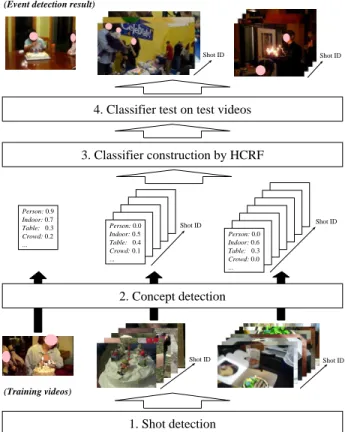
Fig. 1 shows an overview of our concept-based MED method. First, each video is divided into shots using a sim- ple method, where a shot boundary is detected as a signifi- cant difference of colour histograms between two consecu- tive video frames. Then, concepts in each shot are detected.

As a result, we obtain detection scores each of which rep- resents the probability of a concept’s presence in the shot.

In other words, as shown in the middle of Fig. 1, a video is represented as a multi-dimensional sequence where the time index corresponds to shot IDs, and each shot is represented as a vector of concept detection scores. It should be noted that labels of an event’s occurrence or non-occurrence are assigned only to videos. Hence, to overcome this weakly supervised setting as well as the diversity of visual appear- ances, an HCRF is constructed on multi-dimensional se- quences of videos. Below, we describe the concept detec- tion process, and the HCRF construction/test process.

2.1. Concept Detection as Feature Extrac- tion

Since the goal of MED is the development of a gen- eral ad-hoc event detection, features must be extracted and frozen prior to the subsequent event detection. This means that we cannot create features which are specialised to a certain event, that is, we have to use the same features for

1. Shot detection

Person: 0.9 Indoor: 0.7 Table: 0.3 Crowd: 0.2 ...

Shot ID Shot ID

Shot ID Shot ID

2. Concept detection

(Training videos)

3. Classifier construction by HCRF 4. Classifier test on test videos

(Event detection result)

Shot ID Shot ID

Person: 0.0 Indoor: 0.5 Table: 0.4 Crowd: 0.1 ...

Person: 0.0 Indoor: 0.6 Table: 0.3 Crowd: 0.0 ...

Figure 1. An overview of our MED method.

all events. Thus, we need a concept vocabulary that is suf- ficiently rich for describing various events. For this pur- pose, we use Large-Scale Concept Ontology for Multimedia (LSCOM), which is one of the most popular ontologies in the field of multimedia retrieval [5]. LSCOM defines a stan- dardised set of 1, 000 concepts. These are selected based on their ‘utility’ for classifying content in videos, their ‘cover- age’ for responding to a variety of queries, their ‘feasibility’

for automatic detection, and the ‘availability’ (observabil- ity) of large-scale training data.

Our method represents an event as a combination of the above LSCOM concepts. Here, even if there is no concept ‘specific’ to an event, event detection can be per- formed using related concepts. For example, although Birthday Cake and Candle seem very specific to the event

“Birthday party”, they are not defined in LSCOM. In this case, videos containing this event are characterised by re- lated concepts, such as Indoor, Food, Table and Explo- sion Fire.

Annotation data collected by the system in [1] are used

as training examples for constructing detectors of LSCOM

concepts. Roughly speaking, it is unmanageable for few re-

searchers to manually annotate a large number of shots in

terms of each concept’s presence or absence. Thus, the sys-

tem implements Web-based collaborative annotation to dis- tribute manual annotation to many users on the Web. To fur- ther improve annotation efficiency, active learning is used to preferentially annotate shots that are promising for improv- ing the current detector’s performance. The system targets 545, 872 shots in 27, 963 videos in terms of 500 concepts’

presences or absences. These video data and annotation data are used in the Semantinc INdexing (SIN) task [13]

. By analysing collected annotation data, we construct detec- tors of 351 concepts for which more than one positive ex- amples (shots annotated with a concept’s presence) exist.

Concept detection is conducted by the method that we developed at the last year’s SIN task [12]. First, in order to characterise local shapes of objects ( e.g., corners of build- ings, vehicles, human eyes etc.), we extract Scale-Invariant Feature Transform (SIFT) descriptors that characterise edge shapes of local regions, detected by Harris-Affine region de- tector [4]. In such regions, pixel values largely change in multiple directions, so they can be regarded as useful for characterising local shapes of objects. Then, each shot is represented using the GMM-SuperVector (GMM-SV) rep- resentation, which models the distribution of SIFT descrip- tors using a Gaussian Mixture Model (GMM) [3]. Com- pared to the traditional Bag-of-Visual-Words (BoVW) rep- resentation based on the pre-specified template, the GMM- SV is more flexible where a GMM of each shot is adap- tively estimated based on SIFT descriptors. In addition, the GMM-SV can represent variances of SIFT descriptors, which cannot be represented by the BoVW.

Finally, using positive and negative examples for each concept, a Support Vector Machine (SVM) with RBF ker- nel is constructed as a concept detector. Here, randomly selected shots are used as negative examples. Since the con- cept is present only in a small number of shots, almost all of randomly selected shots do not show it and can serve as negative examples [7]. Compared to this, although anno- tation data collected by [1] contain negative examples, our preliminary experiment showed that they lead to worse per- formance than randomly selected shots. One main reason is that negative examples are similar to positive examples, be- cause of the ‘biased’ shot selection by active learning (users are asked to annotate shots similar to already collected pos- itive examples). In contrast, negative examples by ‘non- biased’ random shot selection yield more accurate concept detection.

In the above concept detection, our method in [12] ad- dresses the following two issues: First, a concept is not necessarily present in all videos frames in a shot. To cover this ‘uncertainty’ of the concept’s presence, it is required to exhaustively extract SIFT descriptors from many video frames. Actually, it is reported that, compared to a method

1

We have these data because of our last year’s participation in the SIN task [12].

using features only from one video frame in each shot, a method using features from every 15 frames is more ac- curate by 7.5 to 38.8% [15]. Second, a concept’s appear- ances in shots are significantly different depending on cam- era techniques and shooting environments. Hence, to cover this diversity of the concept’s appearances, a large number of training examples are required. In general, the perfor- mance is proportional to the logarithm of the number of pos- itive examples, although each concept has its own complex- ity [6]. This means that 10 times more positive examples improve the performance by 10%.

However, it requires expensive computational costs to process a huge number of SIFT descriptors for GMM-SV extraction and a large number of training examples for con- cept detection. Thus, we developed a fast GMM-SV extrac- tion method and a fast concept detection method based on matrix operation [12]. The former re-formulates the prob- ability density computation in a GMM, so that probabil- ity densities of many SIFT descriptors can be computed in batch. The latter re-formulates the similarity (kernel value) computation in SVM training and test, which enables batch computation of similarities among many training examples.

Based on these, the GMM-SV extraction and concept de- tection become about 5-7 and 10-37 times faster than the normal implementation, respectively. Owing to this, the GMM-SV of each shot (in both SIN and MED videos) is computed by extracting SIFT descriptors from every other frame. And, each concept detector is constructed using 30, 000 training examples.

2.2. Event Detection by HCRF

Fig. 2 illustrates an HCRF that is constructed using videos represented as multi-dimensional sequences of con- cept detection scores. Assume M videos labelled with an event’s occurrence and N videos labelled with its non- occurrence are given as training videos. For the simplicity, the former and latter videos are called positive videos and negative videos, respectively. Each video x is represented as a multi-dimensional sequence of K concepts’ detection scores, that is, if x has T shots, x = {x

, · · · , x

} where x

= (x

, · · · , x

). Fig. 2 depicts how to determine the event label y ∈ {0, 1} of x, where 0 and 1 mean the event’s non-occurrence and occurrence, respectively. Specifically, x

is first assigned to a hidden state h

∈ H, where H is the set of hidden states. Then, y is determined by combin- ing h = {h

, · · · , h

} assigned to x. Thus, hidden states work as mediators between concept detection scores and an event label. It is known that a model with hidden states has a more powerful discrimination power than a model only using observable values.

Compared to well-known generative models such as

Hidden Markov Models (HMMs), HCRFs have the follow-

Person: 0.9 Indoor: 0.7 Table: 0.3 Crowd: 0.2 ...

Person: 0.9 Indoor: 0.2 Table: 0.1 Crowd: 0.0 ...

Person: 0.4 Indoor: 0.8 Table: 0.5 Crowd: 0.1 ...

Person: 0.8 Indoor: 0.7 Table: 0.2 Crowd: 0.4 ...

y

h₁ h₂ h₃ h_T

x₁ x₂ x₃ x_T

Multi-dimension -al sequence State sequence Event label

Figure 2. An illustration of our HCRF model.

ing advantages. First, generative models are usually con- structed so as to maximise the likelihood of positive videos for each label [16]. However, this is not necessarily optimal for discriminating videos with different labels. On the other hand, HCRFs explicitly maximise the conditional probabil- ity of each label, given a multi-dimensional sequence. Sec- ond, due to the tractability of generative models, each time point is regarded as conditionally-independent of the other time points. In other words, a state at a time point is cho- sen only by considering states and their transitions at the previous time point. Compared to this, HCRFs model the conditional probability of the entire sequence using a sin- gle probability distribution, so that long-range dependencies among various time points can be considered. In addition, this probability distribution is flexible where arbitrary fea- ture representations at each time point can be incorporated.

For each training video x with its event label y, an HCRF is modelled based on the following conditional probability of y given x:

P (y|x, θ) = X h

P(y, h|x, θ) = P

h e

h

x

θ

P

y⁰,

h e

h

x

θ

, (1) where the numerator with the fixed y is normalized by the denominator that is the sum of numerators with all y ∈ Y , so that equation (1) can be considered as a conditional prob- ability. In addition, h is marginalised out by taking the sum of P (y, h|x, θ)s over all possible assignments of h to x.

Also, Ψ(y, h, x; θ) parameterised by θ is called a potential function, and used to examine the compatibility among x, h and y. Various user-defined functions can be used for Ψ, which we will discuss later.

In the HCRF, θ is learned by maximising the log- likelihood based on conditional probabilities for each train- ing video x

and its event label y

:

L(θ) = X

i

logP (y

|x

, θ) − ||θ||

2σ

, (2) where the second term is the log of a Gaussian prior of θ

with the variance σ

, and is useful for preventing θ from be- ing over-fit to training videos. As a smaller σ is used, values in θ are more unlikely to be extremely large. We set σ by cross validation on training videos. To obtain the optimal θ

, a gradient ascent method is used where the derivative of equation (2) in terms of each value in θ can be efficiently computed by propagating values of Ψ for each shot in x

and each hidden state h

in both backward and forward di- rections (brief propagation) [9]. After θ

is obtained, the relevance score of each test video x to the event is com- puted as P(y = 1|x, θ

) based on equation (1). The sorted list of test videos in terms of their relevance scores to the event is returned as the MED result.

Finally, we use the following potential function Ψ:

Ψ(y, h, x; θ) = X

i

x

· θ

(h

) (3)

+ X

i

θ

(y, h

) + X

i≥2

θ

(y, h

, h

),

where θ

(h

) examines the compatibility between the vector of concept detection scores x

and the hidden state h

∈ H. Scalars θ

(y, h

) and θ

(y, h

, h

) repre- sent the compatibility between the label y ∈ Y and h

, and the compatibility between y and the transition from h

to h

, respectively. In total, θ to be estimated consists of θ

with K × |H| dimensions, θ

with |Y| × |H|

dimensions, and θ

with |H| × |H| dimensions.

3. Experimental Results

Our shot detection method detected 51, 857, 32, 384, 180, 219 and 670, 397 shots for videos specified by event kits, background training videos, MED Test Background Search Set, and Progress Search Set, respectively. For all of shots, detection scores for 351 concepts are computed using the method in Section 2.1. Then, an HCRF is con- structed using 100 positive videos defined by the event kit, and negative videos including miss videos defined by this kit and 4, 992 background training videos.

We found that HCRFs are very sensitive to the parameter σ and initial values of θ. For the former, we first prepare the set of possible σs as {2

, 2

, · · · , 2

}. Then, the optimal σ is selected by the following cross validation. The set of training videos is divided into two parts with the same size, where the one is used to construct an HCRF with each σ, the other is used to validate it. Then, we select the σ which yields the HCRF with the highest average precision, and construct the final HCRF using all training videos and the selected σ.

For initial values of θ, we borrow the idea of the ini-

tialisation used in HMMs [16]. The basic idea is to first

perform the ‘hard-assignment’ of shots in a video to hid-

den states, where an HCRF is initialised only using the

maximum likelihood sequence of hidden states. Then, the HCRF is refined by conducting the ‘soft-assignment’ where all possible sequences of hidden states are considered based on Equation (1). To this end, we first group all shots in training videos into clusters of shots with similar concept detection scores. Since the number of shots to be clus- tered is more than 30, 000, a fast clustering method based on the repeated-bisecting algorithm [17] is employed. Starting with a single cluster containing all shots, the cluster with the lowest similarity between shots and the centre, is itera- tively divided into two separate clusters. Then, each cluster centre is regarded as θ

of a hidden state. Furthermore, for each training video, the maximal likelihood sequence of hidden states is computed using dynamic programming technique. Initial values of θ

are determined by count- ing how many shots in positive (or negative) videos are as- signed to each hidden state. Initial values of θ

are set by counting how many transitions occur between two con- secutive shots in positive (or negative) videos. Here, the number of shots in negative videos is much larger than the one in positive videos. Thus, to initialise θ

and θ

, each shot and each transition are weighted by the inverse of the number of shots in positive (or negative) videos.

For our submitted run SiegenKobeMuro MED13 Visual- Sys PROGAll PS 100Ex 6 on the Progress Search Set, we only know the Mean of Average Precisions (MAP) for 20 events (4.1%). In addition, ground truth data are not re- leased for the set. Hence, it is difficult to closely evaluate our MED method. The following discussions are based on results on MED Test Background Set.

3.1. Effectiveness for Weakly Supervised Setting

In order to examine the effectiveness of HCRFs for weakly supervised setting, we compare them to the follow- ing SV M

using the ‘average-pooling’ of concept de- tection scores. In SV M

, concept detection scores in shots in a video are averaged, so that videos with differ- ent numbers of shots can be represented as vectors with the same dimensionality. Then, an SVM with RBF ker- nel is constructed using the same set of training videos to HCRFs. The above average-pooling is adopted in a state- of-the-art MED method [10]. Using SV M

as our base- line, we tested the following three HCRFs. The first one HCRF

uses 10 hidden states and the parameter σ is determined by cross validation. However, a bad result may be obtained by a wrongly determined σ, which makes it dif- ficult to appropriately evaluate the effectiveness of HCRFs.

Thus, the second HCRF

constructs classifiers with 10 hidden states using all possible σs, and manually select the best result. The last HCRF

uses 20 hidden states and the same exhaustive search of σ to HCRF

.

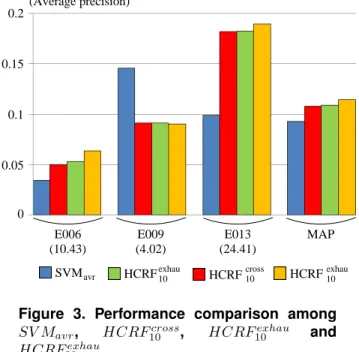
Fig. 3 shows the performance comparison among SV M

, HCRF

, HCRF

and HCRF

. From the left, three sets of four bars represent performances for “E006: Birthday party”, “E009: Getting a vehicle un- stuck” and “E013: Parkour”, respectively. For each set, four bars from the left depict Average Precisions (APs) of SV M

, HCRF

, HCRF

and HCRF

, respectively. The right-most set of four bars represents their MAPs on the above three events. As can be seen from Fig. 3, MAPs of HCRF

, HCRF

and HCRF

are higher than that of SV M

. This val- idates the effectiveness of HCRFs for weakly supervised setting.

E006 (10.43)

E009 (4.02)

E013 (24.41)

MAP 0

0.05 0.1 0.15 0.2

(Average precision)

SVM

HCRF

HCRF

HCRF

Figure 3. Performance comparison among SV M

, HCRF

, HCRF

and HCRF

.

Furthermore, Fig. 3 presents that HCRF

,

HCRF

and HCRF

work much better than

SV M

for E006 and E013, while for E009, the latter

works much better than the formers. One main reason

can be considered as the number of shots in videos where

an event occurs. For each event in Fig. 3, the number in

the parenthesis represents the average number of shots in

videos where this event occurs. Fig. 3 indicates that HCRFs

are very effective for events, which are contained in videos

with many shots. On the other hand, for events which

are contained in videos with a small number of shots, the

average-pooling does not lose much information, and a

non-linear SVM can construct a more precise classifier

than HCRFs, where each hidden state is based mainly on a

linear combination of concept detection scores.

3.2. Evaluation for the Diversity of Visual Appearances

We examine whether HCRFs appropriately cover the diversity of visual appearances in shots relevant to an event. First, we investigate how the performance of HCRFs changes depending on numbers of hidden states. Fig. 4 shows the transition of HCRFs’ performances using 5, 10 and 20 hidden states. The horizontal and vertical axes rep- resent the number of hidden states and AP, respectively. The line overlaid by cross marks depicts the transition of MAPs on three events, and each of the other lines presents the tran- sition of APs on a single event. As can be seen from Fig. 4, as the number of hidden states increases, the performance is improved. This means that more diverse visual appearances are covered by a larger number of hidden states. However, considering the computational cost, using 10 hidden states seems a reasonable choice.

0 0.05 0.1 0.15 0.2

10

5 20

(Average precision)

(Number of hidden states)

E006 E009

E013 MAP

Figure 4. Performance comparison depend- ing on numbers of hidden states.

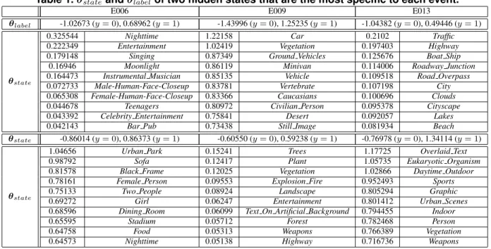
Now, we check whether hidden states appropriately char- acterise concepts relevant to each event. Table 1 represents the two most specific hidden states, that is, these states are associated with the largest values of θ

(y = 1, h) (h ∈ H). In Table 1, 10 rows under the row of θ

present the 10 most characteristic concepts of each hid- den state. These concepts are associated with the largest θ

(h) values, which are shown in the left side of con- cept names. As seen from Table 1, HCRFs appropriately identify relevant concepts to an event, for instance, Night- time and Entertainment for E006 (candle fire is blown in a dark scene), Car and Desert for E009 (a car often gets unstuck on an unstable ground), and City and Sports for E013 (a person does acrobatic performance in a scene with many buildings). However, θ

(h) values wrongly be- come large for some irrelevant concepts. Event detection

performance may be further improved by improving the pa- rameter estimation method as well as the concept detection method,

3.3. Other Issues of HCRFs

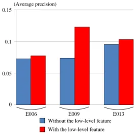
In our concept-based MED method, if there is no con- cept that is very specific to an event, event detection is con- ducted only using related concepts. Although this works reasonably well as shown in Fig. 3, the performance may be further improved if we use low-level features that are very specific to positive videos of the event. Regarding this, considering the computational cost of HCRFs, the 16, 384- dimensional GMM-SV shot representation (used in concept detection) is projected into a 300-dimensional vector using Principle Component Analysis (PCA). Then, this is con- catenated with the 351-dimensional vector of concept de- tection scores. Finally, HCRFs are constructed on multi- dimensional sequences of 651-dimensional vectors.

0 0.05 0.1 0.15

(Average precision)

E006 E009 E013

Without the low-level feature With the low-level feature

Figure 5. Performance comparison between HCRFs with and without the low-level feature.

Fig. 5 presents the performance comparison between HCRFs with the low-level feature and the ones without it.

For each event, APs of the former and latter are represented

by the left and right bars, respectively. As can be seen from

Fig. 5, the low-level feature improves performances for all

events. In the future, we plan to develop a fast HCRF con-

struction method using a parallelisation technique, so that a

precise low-level feature with a large dimensionality can be

incorporated into HCRFs.

Table 1. θ

and θ

of two hidden states that are the most specific to each event.

E006 E009 E013

θ

-1.02673 (y = 0), 0.68962 (y = 1) -1.43996 (y = 0), 1.25235 (y = 1) -1.04382 (y = 0), 0.49446 (y = 1)

θ

0.325544 Nighttime 1.22158 Car 0.2102 Traffic

0.222349 Entertainment 1.02419 Vegetation 0.197403 Highway

0.179148 Singing 0.87349 Ground Vehicles 0.125676 Boat Ship

0.16946 Moonlight 0.86119 Minivan 0.114006 Roadway Junction

0.164473 Instrumental Musician 0.85135 Vehicle 0.109518 Road Overpass

0.072733 Male-Human-Face-Closeup 0.83781 Vertebrate 0.107198 City

0.065308 Female-Human-Face-Closeup 0.83366 Caucasians 0.100696 Clouds

0.044678 Teenagers 0.80972 Civilian Person 0.095378 Cityscape

0.043392 Celebrity Entertainment 0.75841 Desert 0.092057 Lakes

0.042143 Bar Pub 0.73438 Still Image 0.081934 Beach

θ

-0.86014 (y = 0), 0.86373 (y = 1) -0.60550 (y = 0), 0.59238 (y = 1) -0.76978 (y = 0), 1.34114 (y = 1)

θ

1.04656 Urban Park 0.15241 Trees 1.17725 Overlaid Text

0.98792 Sofa 0.12417 Plant 1.05735 Eukaryotic Organism

0.81578 Black Frame 0.12025 Vegetation 1.02866 Daytime Outdoor

0.78161 Female Person 0.09553 Explosion Fire 0.952493 Sports

0.75133 Two People 0.08924 Landscape 0.805294 Graphic

0.69272 Girl 0.06247 Entertainment 0.801412 Urban Scenes

0.68596 Dining Room 0.06099 Text On Artificial Background 0.794455 Indoor

0.65595 Stadium 0.05712 Forest 0.782468 Person

0.64758 Food 0.05313 Weapons 0.766389 Vegetation

0.64573 Nighttime 0.05138 Highway 0.716736 Weapons

4. Conclusion and Future Work

In this paper, we introduced our concept-based MED method using HCRFs. First, every video is represented as a multi-dimensional sequence, where each shot is defined as a vector of concept detection scores. Then, an HCRF is constructed to overcome weakly supervised setting and the diversity of visual appearances in shots. In the HCRF, shots in a video are assigned to hidden states, each of which represents the compatibility between a vector of concept de- tection scores and an event label. Experimental results on MED Test Background Search Set show the effectiveness of HCRFs compared to SVMs. In addition, hidden states can appropriately discriminate between relevant and irrelevant shots to an event, and the diversity of visual appearances can be covered using multiple hidden states.

In the future, we will address the following three issues to improve the performance. First, due to the time limi- tation and the very large size of video data, our current method only uses one image feature (SIFT). Thus, by ex- tracting all features (RGB SIFT, motion, and audio) used in our last year’s SIN method [12], we will improve the per- formance of concept detection, which will lead to the im- provement of event detection. Second, the current HCRF’s parameter estimation takes long computational time. The reason is that the gradient ascent method requires many it- erations, in each of which shots in all training videos have to be checked to obtain the derivative of parameters. Hence, we plan to parallelise the parameter estimation process us- ing multiple processors, each of which processes shots in a subset of training videos.

Finally, in general HCRFs, long-range dependencies among shots are treated by a window approach, where vectors of concept detection scores for consecutive shots are combined into a large-dimensional vector. However, this causes a significant increase of the number of param- eters to be estimated (i.e., the dimensionality of θ

), which in turn requires prohibitive computational cost. To overcome this, the method that we developed in [11] will be used, where the continuity of each concept’s presence over consecutive shots is modelled based on time series segmentation. Then, only the vector where each dimension represents the continuity of a concept’s presence, is incor- porated into HCRFs.

Acknowledgement

We greatly thank Mr. Takumi Origuchi for his intensive collaboration on experiments in this paper.

References

[1] S. Ayache and G. Qu´ enot. Video corpus annotation using ac- tive learning. In Proceedings of the 30th European Confer- ence on Information Retrieval (ECIR 2008), pages 187–198, 2008.

[2] K. Grauman and B. Leibe. Visual Object Recognition. Mor- gan & Claypool Publishers, 2011.

[3] N. Inoue and K. Shinoda. A fast and accurate video semantic-indexing system using fast MAP adaptation and GMM supervectors. IEEE Transactions on Multimedia, 14(4):1196–1205, 2012.

[4] K. Mikolajczyk, T. Tuytelaars, C. Schmid, A. Zisserman,

J. Matas, F. Schaffalitzky, T. Kadir, and L. Gool. A com-

parison of affine region detectors. International Journal of Computer Vision, 65(1-2):43–72, 2005.

[5] M. Naphade, J. Smith, J. Tesic, S.-F. Chang, W. Hsu, L. Kennedy, A. Hauptmann, and J. Curtis. Large-scale con- cept ontology for multimedia. IEEE MultiMedia, 13(3):86–

91, 2006.

[6] M. R. Naphade and J. R. Smith. On the detection of semantic concepts at TRECVID. In Proceedings of the 12th annual ACM international conference on Multimedia (MM 2004), pages 660–667, 2004.

[7] A. P. Natsev, M. R. Naphade, and J. Teˇsi´c. Learning the se- mantics of multimedia queries and concepts from a small number of examples. In Proceedings of the 13th annual ACM international conference on Multimedia (MM 2005), pages 598–607, 2005.

[8] P. Over, G. Awad, M. Michel, J. Fiscus, G. Sanders, W. Kraaij, A. F. Smeaton, and G. Qu´ enot. Trecvid 2013 – an overview of the goals, tasks, data, evaluation mechanisms and metrics. In Proceedings of TRECVID 2013. NIST, USA, 2013.

[9] A. Quattoni, S. Wang, L. Morency, M. Collins, and T. Dar- rell. Hidden conditional random fields. IEEE Transactions on Pattern Analysis and Machine Intelligence, 29(10):1848–

1852, 2007.

[10] R. Aly et al. AXES at TRECVid 2012: KIS, INS, and MED.

In Proceedings of TREC Video Retrieval Evaluation Work- shop (TRECVID 2012), 2012.

[11] K. Shirahama and K. Uehara. A novel topic extraction method based on bursts in video streams. International Jour- nal of Hybrid Information Technology (IJHIT), 1(3):21–32, 2008.

[12] K. Shirahama and K. Uehara. Kobe university and Muroran institute of technology at TRECVID 2012 semantic indexing task. In Proceedings of TREC Video Retrieval Evaluation Workshop (TRECVID 2012), 2012.

[13] A. F. Smeaton, P. Over, and W. Kraaij. Evaluation cam- paigns and TRECVid. In Proceedings of the Eighth Interna- tional Workshop on Multimedia Information Retrieval (MIR 2006), pages 321–330, 2006.

[14] C. G. M. Snoek and M. Worring. Concept-based video re- trieval. Foundations and Trends in Information Retrieval, 2(4):215–322, 2009.

[15] C. G. M. Snoek, M. Worring, J.-M. Geusebroek, D. Koelma, and F. Seinstra. On the surplus value of semantic video anal- ysis beyond the key frame. In Proceedings of IEEE Inter- national Conference on Multimedia and Expo 2005 (ICME 2005), pages 386–389, 2005.

[16] Young S. et al. The HTK Book (for HTK Version 3.4). Cam- bridge University Engineering Department, 2009.

[17] Y. Zhao and G. Karypis. Evaluation of hierarchical clus-

tering algorithms for document datasets. In Proceedings

of the eleventh international conference on Information

and knowledge management (CIKM 2002), pages 515–524,

2002.