Multiperiod Portfolio Selection with Second-order Cone Constraints

Multiperiod Portfolio Selection with Second-order Cone Constraints

Guidance

Professor Masao FUKUSHIMA Assistant Professor Nobuo YAMASHITA

Tomoyuki ITO

1999 Graduate Course in

Department of Applied Mathematics and Physics Graduate School of Informatics

Kyoto University

February 2001

Abstract

The multiperiod portfolio selection model has attracted much attention in the financial

field, because a portfolio is usually rebalanced dynamically in order to get a desired return

even if the situation changes in the future. The scenario tree model is a popular multiperiod

model which consists of many “scenario paths”. However, this model has the disadvantage

that scenario paths grow explosively if we try to describe future situations in detail. In

this paper, in order to overcome this disadvantage, we propose a model that allows returns

on assets at each node to vary in a certain region, rather than increasing the number of

branchings at each node of the scenario tree. The model can deal with shortfall risks in

the case where the worst situation occurs in the region. We formulate the proposed model

as a second-order cone programming (SOCP) problem, which can be efficiently solved by

using the interior point method. Finally, we present some numerical results to show the

usefulness of the proposed model.

Contents

1 Introduction 1

2 Conventional Scenario Tree Model 3

3 The Proposed Models 7

3.1 The model securing floors at each node . . . . 7 3.2 The model securing floors on each scenario . . . . 8 3.3 The model treating asymmetric returns . . . . 9

4 Numerical Experiments 12

4.1 The model used in the experiments . . . 12 4.2 Numerical results . . . 13

5 Conclusion 17

A Second-Order Cone Programming (SOCP) 19

1 Introduction

Recently, many regulations on the financial investment have been relaxed dramatically, especially in Japan. This movement has made it possible for investors to control the allocation of their fund in a more flexible manner. On the other hand, the investors are asked to actively take risks for getting certain returns, because the interest rates have been kept in a low level in Japan. Under such circumstances, the risk management in investments has become increasingly important. Furthermore, mathematical approaches have gradually been recognized as useful tools for the risk management, not only in the academic field but also in the practical field. The purpose of this paper is to propose a model which is useful in constructing a low risk portfolio. To this end, we aim to extend the scenario tree model, which is one of popular multiperiod models for portfolio selection, by introducing the second-order cone constraints.

Until now, various mathematical models have been proposed to formulate the portfolio selection problem. Those models may be classified into two categories, the single-period model and the multiperiod model, from the number of decision making opportunities in the investment period. The single-period model, such as Mean-Variance model by Markowitz [4] and CAPM model by Sharpe [12], have had significant effect on the real investment in business. On the other hand, numerous papers about multiperiod models have appeared since the framework of multiperiod models was introduced by Merton [5, 6]

and Samuelson [11]. As to these two models, it is known that the optimal portfolio obtained by solving a single-period model repeatedly is the same as that obtained by solving a multiperiod model, provided that the distribution of the returns on assets at each period is independently and identically distributed (i.i.d) and the investor’s utility function satisfies some assumptions [7]. However, if the distribution of the returns on assets varies with period, the optimal portfolio in the multiperiod model may differ from the one in the single-period model, because the optimal portfolio in the multiperiod model has a factor of hedging against changes in the state variables. In fact, the analysis using real market data shows that the optimal portfolio in the multiperiod model differs from that of the single-period model [1, 2].

Multiperiod decision making has become an important subject in the practical invest- ment as well as in the academic research on finance. One of the typical examples is the investment for pension funds, of which investment period is so long that the economic sit- uation may change drastically. The investors of the pension fund are asked to get a certain return under any situation, so that they have to take various scenarios into account in advance. Therefore, the investors should rebalance their asset allocation according to the change of the economic situation during the investment period. This practical requirement supports the significance of the multiperiod model.

If we know the distribution of the returns on assets in advance, then we can formulate

the multiperiod model as a stochastic programming problem [6]. However, this problem is difficult to deal with, because the wealth at each period is expressed as the product of random variables that represent the rate of return on asset. Moreover, we need strong assumptions on the distribution of the returns on assets for getting an optimal solution of this problem. Therefore, it is helpful to consider approximation to the multiperiod model.

The scenario tree model approximates the distribution of the returns on assets at each period by a discrete distribution.

Although the scenario tree model has the advantage that it allows us to make decision according to the progress of situations, it has the disadvantage that we cannot describe situations in detail because the number of scenarios increases explosively as the number of branchings at each node increases. In this paper, we propose a model that does not suffer from this disadvantage of the multiperiod scenario tree model. The basic idea underlying the proposed model is as follows. Unlike the conventional scenario tree model, we regard the rate of return on each asset as a parameter which varies in a certain region.

Furthermore, we are particularly interested in the case where the rate of return on the whole portfolio becomes worst when the return on each asset varies in such a region. To translate this idea into action, we add a special constraint to the conventional scenario tree model. The constraint requires the wealth to be greater than a certain constant, even if the worst case occurs. By using this constraint, we can cover the situation which cannot be dealt with in the conventional scenario tree model. We represent this constraint as a second-order cone constraint. Therefore, the proposed scenario tree model is formulated as a Second-Order Cone Programming (SOCP) problem, which may be written as follows:

minimize f

x

subject to A

x + b

≤ c

x + d

i = 1, . . . , N (1.1) F x = g,

where x ∈ R

is the decision variable, f ∈ R

, A

∈ R

, b

∈ R

, c

∈ R

, d

∈ R, F ∈ R

, g ∈ R

are problem parameters and denotes transpose. We can solve this problem efficiently by using the interior point method.

This paper consists of five sections. In Section 2, we describe the conventional for-

mulation of the multiperiod scenario tree model. In Section 3, we propose three models

that involve second-order cone constraints. In Section 4, we report some numerical results

for one of these models, and show the usefulness of the second-order cone programming

formulation. In Section 5, we conclude this paper with some remarks.

2 Conventional Scenario Tree Model

In this section, we review the conventional formulation [14] of the scenario tree model.

Throughout we suppose the following situations. The investor invests his/her wealth during T periods. That is, with the initial wealth W

, the investor first allocates W

to n assets, and then rebalances his/her assets at discrete time periods t = 1, . . . , T − 1.

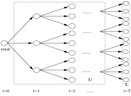
Finally he/she gets a terminal wealth at time t = T . We call the initial time t = 0 the beginning period, the intermediate times t = 1, . . . , T − 1 the internal periods, and the final time t = T the ending period. We suppose that the investor knows possible future situations that may occur from the current situation, but does not know precisely which situation actually occurs. The situation changes from the beginning period to the ending period. We call the path of these situations a scenario. Note that some scenarios may have the same situations up to a certain period. These scenarios cannot be identified until we reach that period. Therefore, the investment strategy on these scenarios must be the same up to that period. From this reason, the progress of the situation can be expressed as a tree with height T (see Figure 1). In the scenario tree, nodes represent all possible situations that may occur in the future. We classify these nodes into three categories according to the height which corresponds to the time, that is, root node v

(t = 0), internal nodes (t = 1, . . . , T − 1) and leaf nodes (t = T ). We use the following notations.

V : The set of all nodes

L ⊂ V : The set of nodes at the ending period, that is, the set of leaf nodes U ⊂ V : The set of nodes at the internal periods

v

∈ V : The node at the beginning period, that is, the root node π

∈ R

: The portfolio at node v

W

∈ R : The wealth at node v

R ¯

∈ R

: The returns on assets when the node v occurs p

∈ [0, 1] : The probability that the node v occurs h(v) : The time when node v occurs

w(v) : The parent node of node v

I

∈ R : The additional fund (> 0) or the consumption (< 0) at node v θ ∈ R : The target wealth at the ending period

Here, we assume

• The probability p

is known for each v ∈ V ;

• The return ¯ R

∈ R

on assets is known for each v ∈ V ;

• The target wealth at the ending period θ is given.

...

...

...

t=0 t=1 t=2 ... t=T

U root

...

L

Figure 1: Scenario Tree Under these assumptions, we consider the risk given by

v∈L

p

( max { 0, θ − W

} )

, (2.1) where k is a positive integer. This risk measure is called the lower partial moment of dimension k. The model based on this risk measure is called the Mean Lower Partial Moment model (MLPM model). Moreover, when the target wealth θ is replaced with

v∈L

p

W

and k = 2, the lower partial moment reduces to the lower semi-variance.

Recent studies [3, 9] prove that the mean standard semideviation (square root of semi- variance) model has a higher consistency with the expected utility theory than mean deviation model.

Now, we consider the problem of finding a portfolio π

(v ∈ { v

} ∪ U ) which minimizes the lower partial moment with k = 2

v∈L

p

( max { 0, θ − W

} )

, (2.2)

under the following two constraints: (i) The expected wealth in the ending period must

be no less than a certain amount α. (ii) The investment in each node must satisfy the

budget constraints on funds. In the multiperiod model, the budget constraints at each

node depend on the investment action in the previous period. Therefore, the budget

constraints at each node depend on the time h(v). We consider the budget constraints for

each node in detail. Let φ : R

→ R be a transaction cost function. That is, φ(π

− π

)

is the transaction cost when the investor rebalances his/her portfolio from π

to π

. To

simplify the discussion, we assume that the transaction cost function is separable, that is, it can be expressed as φ(π

− π

) =

φ

((π

)

− (π

)

), where φ

: R → R, i = 1, . . . , n. Moreover, we assume that the transaction cost φ

((π

)

− (π

)

) on each asset i is linear. Therefore, it is expressed as φ(π

− π

) = a

(π

− π

), where the vector a ∈ R

denotes the transaction cost of each asset. Then we may specify the budget constraints for each period as follows:

Asset allocation at the beginning period : The investor allocates his/her initial wealth W

on the root node v

. So the budget constraint is written as

e

π

= W

, (2.3)

where e is the n-dimensional vector whose entries are all 1.

The wealth and rebalancing at each internal period : At node v ∈ U , the investor obtains the wealth W

which is determined by the portfolio at the parent node w(v).

The wealth at node v therefore can be expressed as

W

= ¯ R

π

. (2.4)

Furthermore, when the investor allocates his/her wealth on assets at node v ∈ U , he/she has to pay the transaction cost φ(π

− π

) incurred by the rebalance. The investor may also add new fund I

> 0 or consume a part of his/her wealth I

< 0.

Therefore, the budget constraint at node v ∈ U is given by

e

π

+ φ(π

− π

) = W

+ I

. (2.5) The wealth at the ending period : The investor no longer rebalances his/her portfo-

lio at node v ∈ L. So, the constraint at the ending period is simply written as

W

= ¯ R

π

. (2.6)

Now we formulate the problem of minimizing the risk given by (2.2) under the con- straints (2.3), (2.4), (2.5) and (2.6):

minimize

v∈L

p

(max { 0, θ − W

} )

subject to

v∈L

p

W

≥ α

e

π

= W

root

e

π

+ φ(π

− π

) = W

+ I

W

= R ¯

π

v ∈ U

W

= ¯ R

π

v ∈ L,

where the decision variables are the portfolios π

at nodes v ∈ { v

} ∪ U , and the wealths W

at nodes v ∈ U ∪ L are dependent on π

and the additional funds I

at nodes v ∈ U are given constants. Since it is not convenient to deal with the function max { 0, θ − W

} , we transform this problem into an equivalent problem by using the artificial variables y

, z

∈ R

such that

θ − W

= y

− z

, y

≥ 0, z

≥ 0. (2.7) Then, we can rewrite the above problem as follows:

[Problem 1 ]

minimize

v∈L

p

y

subject to

v∈L

p

W

≥ α

e

π

= W

root

e

π

+ φ(π

− π

) = W

+ I

W

= R ¯

π

v ∈ U W

= R ¯

π

θ − W

= y

− z

, y

≥ 0, z

≥ 0

v ∈ L

Note that this problem is a convex quadratic programming problem. If we use the risk measure max { 0, θ − W

} , instead of max { 0, θ − W

}

, we can formulate the portfolio se- lection problem as a liner programming problem by means of a similar procedure. The liner programming problem is easier to solve than the quadratic programming problem. There- fore, when we deal with many assets, we may employ this risk measure max { 0, θ − W

} .

In Problem 1, the number of nodes and hence the number of decision variables

increase exponentially with the number of periods or branchings of situations. Until now,

various methods, such as the interior point method [15] and the decomposition method

using parallel computing [8, 10], have been proposed for solving Problem 1. However, it

is reported that those methods hardly reach the level of business use [14].

3 The Proposed Models

In this section, we present three models that cover the disadvantage of the conventional scenario tree model.

Since the scenario tree model can reflect the economical trends, it provides a rough strategy of the investment under varying situations. This is the very advantage of the scenario tree model. On the other hand, as mentioned in Section 2, the scenario tree model has the serious disadvantage that it cannot describe future situations in full detail.

To overcome this difficulty, we regard the rate of return on each note as a parameter which varies in a certain region. For each node v, let a set Γ

⊆ R

be defined by

Γ

:= { R ¯

+ H

u | u ≤ 1 } , (3.1) where H

∈ R

is given matrix. We call this set a return set for the node v. We suppose that the rate of return R

at node v should belong to the return set Γ

.

Remark 1 If matrix H

in (3.1) is nonsingular, then R

= ¯ R

+ H

u ∈ Γ

if and only if u

= (R

− R ¯

)

H

(R

− R ¯

) ≤ 1, (3.2) and hence R

belongs to an ellipsoid centered at R ¯

.

Remark 2 If H

is a diagonal matrix with positive diagonal entries σ

, (i = 1, . . . , n), then, R

∈ Γ

satisfies

σ

(R

− R ¯

)

≤ 1, which particularly implies a return on asset i lies in between ( ¯ R

)

− σ

and ( ¯ R

)

+ σ

.

Now, we consider the case where the rate of return R

on the whole portfolio becomes worst when the return R

varies in the return set Γ

. In the following, we will use the same notations as in the previous section.

3.1 The model securing floors at each node

We consider the requirement that the wealth at each node be no less than a certain constant β

. This β

means the lowest acceptable wealth of the investor at node v, and it is called a floor at node v. This requirement may be represented as follows.

[floor constraints] min

Rv∈Γv

R

π

≥ β

v ∈ U ∪ L. (3.3) It is easy to understand the meaning of the constraints, but it is not convenient to deal with. So, we transform the constraints into second-order cone constraints. Since

R

min

R

π

= min

u≤1

( ¯ R

π

+ u

H

π

)

= R ¯

π

+ min

u≤1

u

(H

π

)

= R ¯

π

− H

π

, (3.4)

the constraint (3.3) is rewritten as

R ¯

π

− H

π

≥ β

. (3.5) These constraints are second-order cone constraints.

Adding the constraints (3.5) to Problem 1, we get the problem securing the floors at each node:

[ Problem 2 ] minimize s

subject to s ≥ (diag(p))

y

v∈L

p

W

≥ α

e

π

= W

root

e

π

+ φ(π

− π

) = W

+ I

W

= R ¯

π

v ∈ U θ − W

= y

− z

, y

≥ 0, z

≥ 0

W

= R ¯

π

v ∈ L H

π

≤ R ¯

π

− β

v ∈ U ∪ L,

where y is the vector whose entries are y

(v ∈ L) and diag(p) is the diagonal matrix whose diagonal entries are p

(v ∈ L). This problem is SOCP, and hence it can be efficiently solved by the interior point method.

3.2 The model securing floors on each scenario

In this subsection, we are interested in securing a desired return at the ending period even if the worst case occurs. Let us pay attention to a scenario itself. Since a scenario is a path of situations changing from the beginning period to the ending period, a scenario i can be represented as

τ

= { v

, v(1, i), v(2, i), . . . , v(T, i) } , (3.6)

where v(t, i) ∈ V (t = 1, . . . , T ). We consider the extreme case where the return of

the portfolio π

becomes worst at every node v(t, i) ∈ τ

(t = 1, . . . , T ). In other

words, we suppose that the wealth W

at each node v(t, i) ∈ τ

is no greater than

min

R

π

. Moreover, the budget in the next period is estimated by

the lowest possible wealth. Consequently, the ending wealth W

becomes the worst

among all possible wealths yielded by the scenario τ

. Based on this idea, we give the

following budget constraints.

e

π

= W

root

e

π

+ φ(π

− π

) = W

+ I

W

≤ min

Rv∈Γv

R

π





v ∈ U W

≤ min

Rv∈Γv

R

π

v ∈ L.

(3.7)

Using the equation (3.4), the constraint W

≤ min

Rv∈Γv

R

π

can be rewritten as

W

≤ R ¯

π

− H

π

. (3.8) Replacing the constraints of Problem 1 with (3.7) and using (3.8), we get the following problem.

[ Problem 3 ] minimize s

subject to s ≥ (diag(p))

y

v∈L

p

W

≥ α

e

π

= W

root

e

π

+ φ(π

− π

) = W

+ I

H

π

≤ R ¯

π

− W

v ∈ U H

π

≤ R ¯

π

− W

θ − W

= y

− z

, y

≥ 0, z

≥ 0

v ∈ L

Similarly to Problem 2, we may also add the constraint (3.5) to Problem 3. Then the constraints are given by

e

π

= W

root

e

π

+ φ(π

− π

) = W

+ I

H

π

≤ R ¯

π

− W

v ∈ U H

π

≤ R ¯

π

− W

v ∈ L H

π

≤ R ¯

π

− β

v ∈ U ∪ L.

The combined problem is also SOCP, so this problem can be also solved efficiently [Ap- pendixA].

3.3 The model treating asymmetric returns

In the previous sections, we defined a return set Γ

by using matrix H

. This implies that

the return R

belongs to a symmetric region. However, the distribution of the returns on

assets is generally asymmetric, especially in the case of the derivatives such as options.

Note that an option is the right to buy or sell an asset at the price (strike price) which is determined in advance. So an option holder exercises his/her option only if he/she can profit from it, and he/she abandons it otherwise. That is, the return on the option depends on whether the holder exercises or not. This implies that the distribution of the return on an option is asymmetric.

In such cases, the equality

R

min

R

π

= ¯ R

π

− H

π

is not satisfied in general. Therefore, the wealth in the worst case cannot be expressed as a second-order cone constraint as in the previous subsections. In the following, we describe a return set Γ

by using two diagonal matrices H

and H

, where H

are used for holding assets and H

for shorting assets. Moreover we define H

as

H

= H

0 0 H

. (3.9)

Using this matrix, we define the region Γ

as Γ

= R ¯

− R ¯

+ H

u

u

u = u

u

, u

∈ R

, u

∈ R

, u ≤ 1

. (3.10) Using this return set, we may derive an equation similar to (3.4) for asymmetric returns.

To this end, we represent the portfolio π

on node v as the difference of two nonnegative vectors π

and π

, that is,

π

= π

− π

, π

≥ 0, π

≥ 0. (3.11) Note that π

corresponds to the holding portfolio and π

corresponds the shorting port- folio.

Let

Π

= π

π

. Then we have

R

min

R

Π

= min

u≤1

R ¯

− R ¯

Π

+ u

H

Π

)

= R ¯

− R ¯

Π

+ min

u≤1

u

(H

Π

)

= R ¯

− R ¯

Π

− H

Π

= R ¯

π

− R ¯

π

−

H

π

H

π

= R ¯

π

−

H

π

H

π

. (3.12)

Therefore, we can deal with an asymmetric return distribution by means of second-order cone constraints.

The obtained solution for this case seems to suggest that the investor should buy and sell the same asset at the same time. However, we can show that the portfolio π

obtained from (3.11) is valid even for such assets. To this end, suppose that π

and π

, satisfy the following inequality for a given η > 0:

H

π

H

π

≤ η. (3.13)

Let ˜ π

, π ˜

satisfy (3.11) with (˜ π

)

= 0 or (˜ π

)

= 0 for each i. Here, without loss of generality, we consider ˜ π

= 0. Then, we have π

= ˜ π

, π ˜

≥ 0 and ˜ π

= 0 from (3.11).

Since H

and H

are diagonal matrices, and since 0 ≤ π ˜

≤ π

, we have H

π ˜

≤

H

π

H

π ˜

= 0 ≤

H

π

. By adding these inequalities, we obtain

H

π ˜

0

≤

H

π

H

π

≤ η, (3.14)

where the last inequality follows from (3.13). This implies that (˜ π

, 0) is also a solution

of the problem, indicating the validity of the representation (3.11).

4 Numerical Experiments

In this section, we report some numerical experiments for the proposed model with real market data. First, we will explain how to construct a scenario tree from the real market data. Next we will solve Problem 1 and Problem 2, and compare the obtained solutions from the viewpoint of risk.

4.1 The model used in the experiments

In this subsection, we describe how to construct the scenario tree model used in the numerical experiments from real market data. Moreover, we modify Problem 1 and Problem 2, so that the problems involve the short-sale constraints. The reason is that the optimal solutions of the original Problem 1 and Problem 2 may not be realistic, since the portfolio may include a large amount of short selling.

The scenario tree : In our experiments, we consider three assets; stock, bond and cash.

We assume that the returns on these assets follow a multivariate normal distribution.

We estimate the mean vector µ ∈ R

of the three assets, and the variance-covariance matrix Σ ∈ R

from the historical data. The used data are annual returns from 1990 to 2001 in Japanese market. We determine the return on each node of scenario tree by using the multivariate normal distribution with µ and Σ. That is, the price S

(t) (i = 1, 2, 3) of each asset i at each discrete time t (t = 0, 1, . . . , T ) is governed by

∆S(t) = D(t)

µ + (Σ)

ε

, (4.1) where

∆S(t) =







∆S

(t)

∆S

(t)

∆S

(t)







≡







S

(t + 1) − S

(t) S

(t + 1) − S

(t) S

(t + 1) − S

(t)







, D(t) =







S

(t) 0 0 0 S

(t) 0 0 0 S

(t)







with the normal random variable ε ∈ R

. We generate a scenario tree with T = 4.

Each node of the scenario tree has 5 branchings. Therefore, the whole scenario tree has 781 nodes. The rate of the return of each scenario is determined by (4.1).

The return sets Γ

: We give the return sets Γ

used in the proposed model as Γ

:= { R ¯

+ δ (Σ)

u | u ≤ 1 } ,

where Σ is a variance-covariance matrix obtained from the historical data and δ is a positive constant. The reason why we choose Γ

as the return set is as follows. If the return on assets at node v is given by (4.1), then the return on assets is expressed as

R ¯

= µ + (Σ)

ε

,

where ε

denotes a constant vector randomly generated from normal distribution.

So, it is reasonable to expect that R

belongs to the set Γ

.

The short-sale constraints : The short-sale constraints are defined by π

≥ − ν

∀ v ∈ v

∪ U,

where ν

∈ R

is a given vector whose components are nonnegative. This constraint means that the amount of short selling should not exceed ν

. Without these con- straints, the optimal portfolio may include a large amount of short selling, especially in the model that used the historical data in Japan. To avoid unrealistic shorting of assets, we add the short-sale constraints to the original problems. Note that the constraints are liner, and hence adding the constraints to a SOCP does not increase the complexity of the problem.

4.2 Numerical results

To see the usefulness of the proposed model, we made some numerical experiments with the scenario tree constructed as described in the previous subsection, and compared it with the conventional model.

We coded programs with MATLAB Version 5. We solved Problem 2, which is the second order cone problem, by using SeDuMi [13]. Note that SeDuMi is a solver for convex minimization problems on a self-dual cone and it uses the interior point method.

Simulations

First we explain our simulations. In the practical investment, the obtained strategy is used only in the beginning period, and will not be in the future periods. This is because the actual changes of situations are usually different from those predicted initially, and hence it does not make sense to follow the strategy through the remaining periods. In practice, whatever the investor allocates at the beginning period, he/she would consider a new scenario tree in the next period and update the strategy using the revised information.

This procedure is repeated recursively from the beginning period t = 0 to the ending period t = T, and the resulting final wealth is evaluated.

The procedure is as follows.

Step.0 Solve the problem with the scenario tree constructed in the manner explained in the previous subsection, and obtain the portfolio π

. Set t := 1.

Step.1 Generate a sample return R by

R = µ + (Σ)

ε,

where ε is a vector randomly generated from normal distribution, and revise the

wealth by R

π

.

Step.2 If t = T , then terminate with the final wealth R

π

. Otherwise, let the initial wealth be R

π

and solve the problem with T − t investment periods to obtain the updated portfolio π

. Set t := t + 1 and go to Step.1.

In our experiments, we did the above simulations J times for Problem 1 and Problem 2 with the same scenario tree. Let the investor’s final wealth obtained in the j th simulation be W

and define

W ¯ := 1 J

J j=1

max(θ − W

, 0)

. (4.2)

This value means the average of the risks obtained through the simulations. We did the simulations with various values of the parameter α (see below). Note that when the problem was infeasible at a certain period, we did not rebalance the portfolio at that period, and kept holding the portfolio of the previous period.

We used the following values of the parameters.

Investment period T T = 4

The number of assets n n = 3

The number of branchings in each node 5

The initial wealth W

W

= 100

The matrix H

at each node v H

= 0.5 Σ

The floor β

at node v β

= W

The target wealth θ θ = 1.055

W

The number of simulation paths J J = 100

The required expected return α α = (1.03 + 0.0025 k)

W

(k = 1, . . . , 30) The additional fund I

at node v I

= 0

The vector of transaction costs a a = (0.01, 0.005, 0.001)

Results of Simulations

We present the results of simulations in Figures 2, 3, 4 and 5.

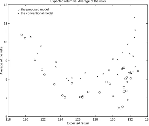
Figure 2 shows the relationship between the average risk ¯ W and the expected return

at the ending period. Figures 3 and 4 show the expected return and the average risk at the

ending period, respectively, for each value of the required expected return α. From Figure

3, we see that the expected return at the ending period in the proposed model is almost

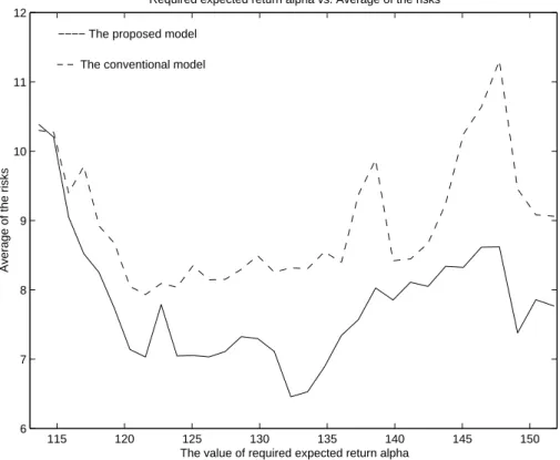
the same as in the conventional model. However, Figure 4 indicates that the proposed

model can reduce the risk compared with the conventional model. From this, we conclude

that the proposed model is useful in finding a portfolio with lower risk. Figure 5 shows

the shortfall risk for each value of the required expected return α. It may be observed

from the figure that the proposed model is also useful in securing the floors.

118 120 122 124 126 128 130 132 134 6

7 8 9 10 11 12

Expected return

Average of the risks

Expected return vs. Average of the risks o the proposed model

x the conventional model

Figure 2: Expected return vs. the average of risks

115 120 125 130 135 140 145 150

118 120 122 124 126 128 130 132 134

The value of required expected return alpha

Expected return

Required expected return alpha vs. Expected return

−−−− The proposed model

− − The conventional model

Figure 3: The required expected return α vs. expected return

115 120 125 130 135 140 145 150 6

7 8 9 10 11 12

The value of required expected return alpha

Average of the risks

Required expected return alpha vs. Average of the risks

−−−− The proposed model

− − The conventional model

Figure 4: The required expected return α vs. the average of risks

115 120 125 130 135 140 145 150

0 0.01 0.02 0.03 0.04 0.05 0.06 0.07 0.08

The value of required expected return alpha

Probability of shortfall from W0

Required expected return alpha vs. probability of shortfall

−−−− The proposed model

− − The conventional model

5 Conclusion

In this paper, we have proposed the model that extends the scenario tree model. The proposed model takes into account the worst return of the portfolio at each node by means of second-order cone constraints and is easy to solve by the interior point method.

Moreover, to show the usefulness of this model, we did some simulations. The numerical results indicate that the proposed model is useful in reducing the shortfall risk.

Finally, we mention further research topics. In the simulations, we assumed that the asset follows the multivariate normal distribution, and we used the squared root of the variance-covariance matrix as H

in the return set Γ

. It may be worth considering how to construct a more practical scenario tree and H

for business use. Another important task we have to do is to deal with models with practical (large) size.

Acknowledgement

I would like to express my sincere appreciation to Professor Masao Fukushima. He care- fully read this thesis and commented in detail on the whole work in this thesis. I would like thank Associate Professor Tetsuya Takine for his helpful comments. His precise com- ments make this paper better than before. I am deeply indebted to Assistant Professor Nobuo Yamashita for his earnest guidance. Without his help, none of the work could be completed. I would like to thank thank all members in Professor Fukushima’s Laboratory for their warm friendship during the course.

References

[1] M. J. Brennan, E. S. Schwartz and R. Lagnado, Strategic asset allocation, Journal of Economic Dynamics and Control 21 (1997), 1377–1403.

[2] J. Campbell and L. M. Viceira, Consumption and portfolio decisions when expected returns are time varying, Quarterly Journal of Economics 114 (1999), 433–495.

[3] H. Konno, Financial engineering II, (in Japanese), Nikkagiren-syuppansya, tokyo, 1998.

[4] H. Markowitz, Portfolio selection: efficient diversification of Investments, John Wiley

& Sons, New York, 1959.

[5] R. C. Merton, Lifetime portfolio selection under uncertainty: The continuous time case, Review of Economics and Statistics 51 (1969), 247–257

[6] R. C. Merton, Optimum consumption and portfolio rules in a continuous-time model,

Journal of Economic Theory 3 (1971), 373–413.

[7] J. Mossin, Optimal multiperiod portfolio policies, Journal of Business 41 (1968), 215–229.

[8] J. M. Mulvey and A. Ruszczynski, A new scenario decomposition method for large- scale stochastic optimization, Operations Research 43 (1995), 477–490.

[9] W. Ogryczak and A. Ruszczynski, From stochastic dominance to mean-risk models:

Semideviations as risk measures, Interim Report 97–027, International Institute for Applied Systems Analysis, Laxenburg, Austria (1997).

[10] T. Rockafellor and R. J. Wets, Scenarios and policy aggregation in optimization under uncertainty, Mathematics of Operations Research 16 (1987), 32–49.

[11] P. A. Samuelson, Lifetime portfolio selection by dynamic stochastic programming, Review of Economics and Statistics 51 (1969), 238–246.

[12] W. Sharpe, Capital asset prices: A theory of market equilibrium under conditions of risk, Journal of Finance 19 (1964), 425–442.

[13] J. F. Sturm, Using SeDuMi 1.02, A Matlab toolbox for optimization over symmetric cones, Optimization Methods and Software 11 & 12 (1999), 625–653.

[14] H. Takehara, optimization of portfolio,(in Japanese), Asakura-Shoten, Tokyo, 1997.

[15] H. Takehara, An interior point algorithm for large scale portfolio optimization, Annals of Operations Research 45 (1993), 373–386.

[16] T. Tsuchiya, A convergence analysis of the scaling-invariant primal-dual path-

following algorithms for second-order cone programming, Optimization Methods and

Software 11/12 (1999), 141–182.