III-2-2. Nature of binomial distribution
III-2-2-1. Probability distribution of binomial distribution
Statistics is a method for estimation of parent population from data population. Most simple and general method is describing histogram. However, we need summarizing the distribution by several characteristics for statistical analysis. Firstly, we consider description of distribution of population.
Definition of necessary terms
Expectation value: Sum of products of the obtainable value and possibility of probability event
𝐸 𝑓(𝑥) = ∑ 𝑓(𝑥 ) 𝑝
Where
𝑓(𝑥 ): obtainable value by event i 𝑝(𝑖): possibility of event i 𝐸 𝑓(𝑥) : expectation value
Formula 9 More practically, average value of obtained values by infinitely repeats of probability event
Average
Definition 1: The value obtained by dividing sum of all data by number of data
∑ 𝑥
𝑛
Definition 2: Expectation value of from obtained data 𝑥 𝑝
𝑥̅ =∑ 𝑥
𝑛 = 𝑥 𝑝
𝑥̅: average of 𝑥
Formula 10 Moment: Value characterizing the distribution of data, calculated as expectation value of (𝑥 − 𝑎)
E(𝑥 − 𝑎) =∑ (𝑥 − 𝑎) 𝑛
When r=1, E(𝑥 − 𝑎) is liner moment When r=2, E(𝑥 − 𝑎) is quadratic moment When 𝑎 = 0, E(𝑥) is moment around origin When 𝑎 = μ, E(𝑥 − 𝜇) is moment around mean
𝜇: mean of parent population
We can say that mean is liner moment around origin and variance is quadratic moment around mean.
SS: Sum of square of the distance of data from average.
SS = (𝑥 − 𝑥̅) 𝑥̅: average of data 𝑛: number of data
Formula 11 There several possible methods for the estimation of mean of parent population such as simulation by repeated random sampling (MCMC, etc). In those methods, distribution of possible mean value can be directly estimated using the power of computer. We consider expectation value of mean of parent population is average of sample population intuitively and estimate mean of parental population by averaging the sample population. We already accept this as axiomatic truth. However, we have to discuss the adequacy of this expectation method from the purpose of estimation of parental population. The reason for the estimation of mean of parent population is that the value shows the most important character of distribution of parent population, center of distribution.
We learned that binomial distribution express by following equation in former chapter, 𝑊(𝑘) = 𝐶 𝑝 𝑞( )
This means that we can draw the shape of binominal distribution when we know the value of 𝑛 and 𝑝 theoretically, because 𝑝 + 𝑞 = 1 . We already know that the shape is unimodal. The position of the peak is most important characteristic of the distribution.
The peak is extreme value and the position is obtainable by solution of following derivation equation.
𝑑𝑊(𝑘) 𝑑𝑘 = 0
However, derivation of 𝐶 𝑝 𝑞( ) by k needs several mathematical techniques, and the process of explanation of the solution long and complicated. We will show another method
to obtain the position of the peak without using derivation in following paragraphs at first, then we will show the solution by derivation in later paragraphs.
It may be understandable sensuously.
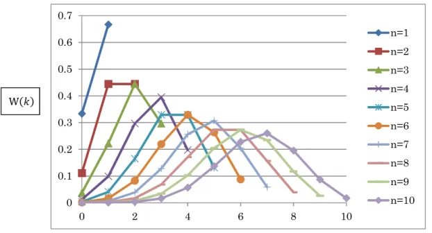
Figure 6 shows relation of 𝑊(𝑘), n and k. when p = . This is expressed B 𝑛, . Taking coin toss game as an analogy, k is times of head and probability of head (A) in a try is , and that of tail (B) is . W(k) is probability of k times head and n-k times tail. or probability of k times A and n-k times B. With the increase of n, the plot expands to right side and peak moves to right with the expand of the plot as shown in Fig 6.
Fig.6. 𝑊(𝑘) = 𝐶 𝑝 𝑞( ), B(n, )
In B(9, ), peak exists at 𝑘 = 6. In B(6, ) peak exists at 𝑘 = 4, and peak exists at 𝑘 = 2 in B 3, . In other cases, the positions of peak is not clear, though the position is
around k where = 𝑝. We may consider that the 𝑘which gives peak is 𝑘 = 𝑛𝑝. Simply, probability of A in a try is and we try two times. So maximum probability is obtained at 𝑘 = + , and when we try 𝑛 times, maximum probability is obtained at 𝑛𝑝. This is the answer to the question “When you know the probability of A in a try and you try n times, how many times A happen? Answer the most probable times”. The answer to this question is expectation value of 𝑘.
𝑘 = 𝑛𝑝. (𝑘: expectation value of 𝑘)
This is still only our prediction. We need to confirm the prediction.
0 0.1 0.2 0.3 0.4 0.5 0.6 0.7
0 2 4 6 8 10
n=1 n=2 n=3 n=4 n=5 n=6 n=7 n=8 n=9 n=10 W(𝑘)
In above mentioned model, number of repeats in a set is 𝑛, and expectation value (𝑘) can be obtained by summing up products of each value and probability
There are 𝑛 + 1 𝑘s; (0, 1, 2, ⋯ 𝑛).
𝑘 = 𝑊(𝑘) × 𝑘
=∑ 𝐶 𝑝 𝑞( )× 𝑘
= 𝑘𝑛!
𝑘! (𝑛 − 𝑘)!𝑝 𝑞( )
= 𝑘𝑛(𝑛 − 1)!
𝑘! ((𝑛 − 1) − (𝑘 − 1))!𝑝 × 𝑝( )𝑞( ) ( ))
𝑘 = 𝑛(𝑛 − 1)!
(𝑘 − 1)! ((𝑛 − 1) − (𝑘 − 1))!𝑝 × 𝑝( )𝑞( ) ( ))
𝑘 = np (𝑛 − 1)!
(𝑘 − 1)! ((𝑛 − 1) − (𝑘 − 1))!𝑝( )𝑞( ) ( ))
∑ ( )!((( )!
) ( ))!𝑝( )𝑞( ) ( )) is a sum of all probability when 𝑛 = 𝑛 − 1.
(𝑛 − 1)!
(𝑘 − 1)! (𝑛 − 1) − (𝑘 − 1) !𝑝( )𝑞( ) ( )) = 1 then
𝑘 = 𝑛𝑝
Q.E.D In a binomial distribution B(𝑛, 𝑝), possibility of 𝑘 times appearance of a phenomenon in 𝑛 trials (𝑊(𝑘)) is as follow
𝑊(𝑘) = 𝐶 𝑝 𝑞( )
= !( ! )!𝑝 𝑞( ) 𝑝 + 𝑞 = 1
When we take logarithm of both members.
logW(𝑘) = log(𝑛!) − log(𝑘!) − log(𝑛 − 𝑘)! + 𝑘 log(𝑝) + (𝑛 − 𝑘) log(𝑞)
The equation becomes linear by the transformation and we can discuss each member separately. Here we consider 𝑘 as continuous valuable (real number, not limited in integer). Generally, 𝑘 is used expression of integer, so we rewrite 𝑘 to 𝑥. This is a custom and wisdom to prevent misunderstanding.
logW(𝑥) = log(𝑛!) − log(𝑥!) − log(𝑛 − 𝑥)! + 𝑘 log(𝑝) + (𝑛 − 𝑥) log(𝑞)
Formula 12 Without any prior information, you need to accept following equation.
lim→ log𝑥! = lim
→ 𝑙𝑜𝑔 𝑡 𝑑𝑡
This equation means that ∫ 𝑙𝑜𝑔 𝑡 𝑑𝑡 ≒logx!, when 𝑥 is large enough. This equation is simple, and you may accept this equation in an intuitive way. We need several mathematical techniques for proper proof of this equation and the process of proof is complicated and boring. The readers who do not like such boring story can skip
following paragraphs. It makes no problem, though it is useful for readers who want to understand what we are doing to make probability models
Proof of
lim→ ∫ 𝑙𝑜𝑔x 𝑡 𝑑𝑡 = lim
→ log 𝑥!
Conclusively, given equation is transformation of following equation. This is our goal.
x→lim
∫ log 𝑡𝑑𝑡1x log 𝑥! = 1 In the symbol of limitation, there is
log 𝑡𝑑𝑡
x
1
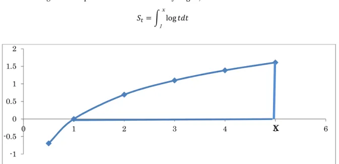
The meaning of this equation is area framed by log 𝑡 , X axis and X = 𝑥.
𝑆 = log 𝑡𝑑𝑡
x 1
Fig 7.1 Integration range of ∫ log 𝑡𝑑𝑡1x
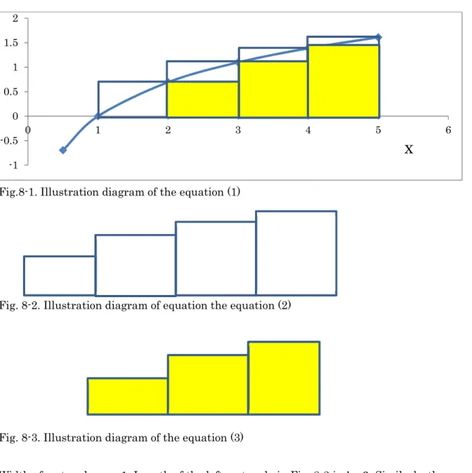
We put several rectangles in the figure. Figure 8-1 is overlap of following 2 figures.
-1 -0.5 0 0.5 1 1.5 2
0 1 2 3 4
x
5 6Fig.8-1. Illustration diagram of the equation (1)
Fig. 8-2. Illustration diagram of equation the equation (2)
Fig. 8-3. Illustration diagram of the equation (3)
Width of rectangles are 1. Length of the left rectangle in Fig. 8-2 is log 2. Similarly, the length of other rectangles are log 3, log 4 and log 5. Sum of 4 rectangles is follow.
S = log 2 + log 3 + log 4 + log 5 = log 5!
When 𝑥 increases,
S = log 𝑥!
Similarly. Sum of the area of yellow rectangles is as follow.
S = log(𝑥 − 1)!
When we focus on the size of the areas. Figure 18-1 shows, S > S > S
log(𝑥 − 1)! < log 𝑡𝑑𝑡
x 1
< log 𝑥!
-1 -0.5 0 0.5 1 1.5 2
0 1 2 3 4 5 6
x
Here,
𝑥 > 1, log 𝑥! > 0
We can divide all members without change of direction of inequality sign .
( )!
! <∫ ! < !! Obviously,
!
!= 1 Then we consider limit of left member.
log(𝑥 − 1)!
log 𝑥! =log(𝑥 − 1) + log(𝑥 − 2) + ⋯ + log 1 log 𝑥!
=log 𝑥 + log(𝑥 − 1) + log(𝑥 − 2) + ⋯ + log 1 − log 𝑥 log 𝑥!
=log 𝑥! − log 𝑥 log 𝑥!
= 1 − log 𝑥 log 𝑥!
For the author, lim != 0 is trivial, though sense of triviality is different among people. It is better to proof
lim→
log 𝑥 log 𝑥!= 0 Proof
log 𝑘! > log 𝑘 + log(𝑘 − 1) + ⋯ + log 𝑘 2 > 𝑘
2− 1) log 𝑘 2 Meaning of above inequality is as follow
k
2 : maximum integer number which does not exceed 𝑘. When 𝑘 = 5, k
2 = 2.
When 𝑘 = 4, k
2 = 2,
log 𝑘! > log 𝑘 + log(𝑘 − 1) + ⋯ + log means that cantle does not exceed entirety.
Log 𝑘! = log 𝑘 + log(𝑘 − 1)! + ⋯ + log 1
log 𝑘 + log(𝑘 − 1) + ⋯ + log 𝑘 2
All members of right side of inequalities are positive.
So
log 𝑘! > log 𝑘 + log(𝑘 − 1) + ⋯ + log 𝑘 2
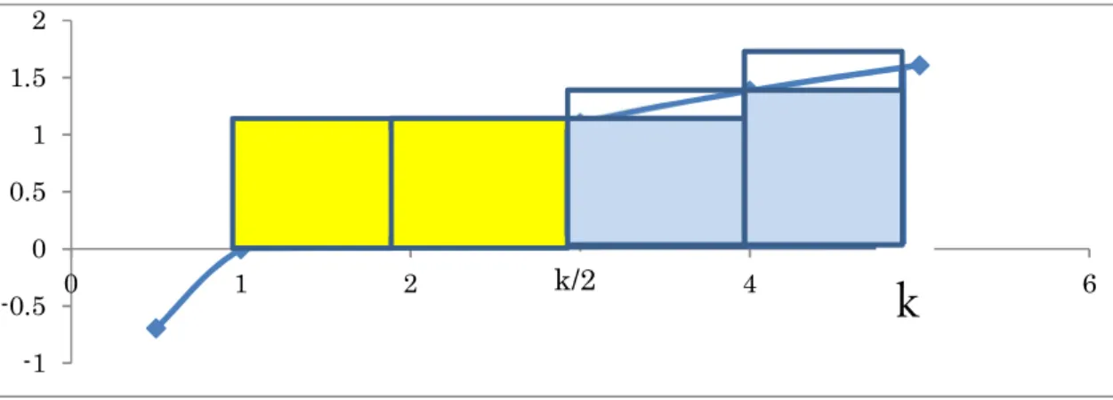
log 𝑘 + log(𝑘 − 1) + ⋯ + log > − 1) log means comparison between sum of the blue rectangles and the sum of the area of yellow rectangles in figure 9.
黄色で示した四角形の面積の総和は、青で示した四角形の面積の総和を超えない。
これで
log 𝑘! > 𝑘
2− 1) log 𝑘 2 を示すことができました。
Fig. 9. Comparison of magnitude relationship.
log 𝑘 + log(𝑘 − 1) + ⋯ + log 𝑘 2 > 𝑘
2− 1) log 𝑘 2 is proven.
And also log 𝑘! > log 𝑘 + log(𝑘 − 1) + ⋯ + log 𝑘
2 > 𝑘
2− 1) log 𝑘 2 is proven.
Conclusively
log 𝑘! > 𝑘
2− 1) log 𝑘 2 log 𝑘! > 𝑘
2− 1) log 𝑘 2 we can transform 𝑘 𝑎𝑠 𝑥,
log 𝑥! > 𝑥
2− 1) log 𝑥 2 The relation is the same when 𝑥 → ∞ .
-1 -0.5 0 0.5 1 1.5 2
0 1 2 k/23 4 5 6
k
lim→ log 𝑥! > lim
→
𝑥
2− 1) log 𝑥 2 When 𝑥 → ∞ , lim
→ − 1) log > 1 lim→
1
log 𝑥!< lim
→
1 𝑥
2− 1) log 𝑥 2
= 0 Here,
log 𝑥 > 0 𝑎𝑛𝑑 1 log 𝑥!> 0 log 𝑥
log 𝑥!> 0
0 ≤ lim
→ !≤ lim
→
x = lim
→ ( )= lim
→ ( )= 0
0 ≤ lim
→
log 𝑥 log 𝑥!≤ 0 lim→
log 𝑥 log 𝑥!= 0
is proven. The method used in above proof is called false position method.
lim→ (1 −log 𝑥 log 𝑥!) = 1 1 − log 𝑥
log 𝑥!=log 𝑥! − log 𝑥
log 𝑥! =log𝑥!
𝑥
log 𝑥!=log(𝑥 − 1)!
log 𝑥!
So
lim→
log(𝑥 − 1)!
log 𝑥! = 1 1 = lim
→
log(𝑥 − 1)!
log 𝑥! ≤ lim
→
∫ log 𝑡𝑑𝑡 log 𝑥! ≤ lim
→
log 𝑥!
log 𝑥!= 1 Using false position method,
x→lim
∫
! =1
x→lim log 𝑡𝑑𝑡 = lim
x→ log 𝑥!
When 𝑥 is large enough,
log 𝑥! ≒ log 𝑡𝑑𝑡 We go back to equation 12
logW(𝑥) = log(n!) − log(𝑥!) − log(𝑛 − 𝑥)! + 𝑥log(𝑝) + (𝑛 − 𝑥) log(𝑞)
≒ log(𝑛!) − log 𝑡𝑑𝑡 − log 𝑡𝑑𝑡 + 𝑥 log 𝑝 + (𝑛 − 𝑥) log 𝑞 In case of 𝑥 → ∞, we can write
logW(𝑥) = log(𝑛!) − ∫ log 𝑡𝑑𝑡 − ∫ log 𝑡𝑑𝑡 + 𝑥 log 𝑝 + (𝑛 − 𝑥) log 𝑞 {log 𝑊(𝑥} = − log 𝑥 + log(𝑛 − 𝑥) + log 𝑝 − log(1 − 𝑝)
= log(𝑛 − 𝑥)𝑝 𝑥(1 − 𝑝) because 𝑑𝑡(𝑡log𝑡 −𝑡)
𝑑𝑡 = 1 ∙ log𝑡 + 𝑡 ∙1
𝑡− 1 = log𝑡
∴ log𝑡𝑑𝑡 = 𝑡log𝑡 −𝑡 + 𝐶
∴ log 𝑡𝑑𝑡 = 𝑥log𝑥 −𝑥 − 1 log 1 + 1 = 𝑥log𝑥 −𝑥 + 1
∴𝑑 ∫ log 𝑡𝑑𝑡
𝑑𝑥 = 1 × log𝑥 +𝑥1
𝑥− 1 = log𝑥 𝑑(log 𝑛!)
𝑑𝑥 = 0,𝑑(𝑥 log 𝑝)
𝑑𝑥 = log 𝑝 ,𝑑 (𝑛 − 𝑥) log 𝑞
𝑑𝑥 = log 𝑞 = log(1 − 𝑝) When
( )
x( )= 1, log(𝑛 − 𝑥)𝑝
𝑥(1 − 𝑝)= 0 (𝑛 − 𝑥)𝑝 𝑥(1 − 𝑝)= 1
∵ log 1 = 0 (𝑛 − 𝑥)𝑝 = 𝑥(1 − 𝑝)
𝑛𝑝 − 𝑥𝑝 = 𝑥 − 𝑥𝑝 𝑥 = 𝑛p
The (log 𝑊(𝑥))′ is monotonically decreasing function and (log 𝑊(𝑥))′ is 0 at 𝑥 = 𝑛p
This result means log 𝑊(𝑥) is local maximum value at 𝑥 = 𝑛p, and the plot of the
probability 𝑊(𝑥)peaks at 𝑥 = 𝑛p
This conclusion agrees with our empirical prediction μ = 𝑛𝑝
For readers who know derivation of composite function, the conclusion is obtainable simply.
Rule of derivation of composite function is as follow 𝑑𝑓 𝑔(𝑥)
𝑑𝑥 =𝑑𝑓 𝑔(𝑥) 𝑑𝑔(𝑥)
𝑑𝑔(𝑥) 𝑑𝑥 Here,
logW(𝑥) = log(𝑛!) − log(𝑥!) − log(𝑛 − 𝑥)! + 𝑥 log(𝑝) + (𝑛 − 𝑥) log(𝑞) W(𝑥) = 𝑒( ( !) ( !) ( )! ( ) ( ) ( ))
𝑔(𝑥) = log(𝑛!) − log(𝑥!) − log(𝑛 − 𝑥)! + 𝑥 log(𝑝) + (𝑛 − 𝑥) log(𝑞) W 𝑔(𝑥) = 𝑒 ( )
𝑑W 𝑔(𝑥)
𝑑𝑔(𝑥) = 𝑒 ( ) 𝑑𝑔(𝑥)
𝑑𝑥 = − log 𝑥 + log(𝑛 − 𝑥) + log(𝑝) − log(𝑞) 𝑑W 𝑔(𝑥)
𝑑𝑥 =𝑑W 𝑔(𝑥) 𝑑𝑔(𝑥)
𝑑𝑔(𝑥)
𝑑𝑥 = 𝑒 ( )(− log 𝑥 + log(𝑛 − 𝑥) + log(𝑝) − log(𝑞))
=𝑒 ( ) log(( )) Calculation of 𝑥 which gives extreme value
𝑑W 𝑔(𝑥)
𝑑𝑥 = 𝑒 ( ) log(𝑛 − 𝑥)𝑝 𝑥(1 − 𝑝) = 0 𝑒 ( ) > 0 (𝑛𝑜𝑡 0)
(𝑛 − 𝑥)𝑝 𝑥(1 − 𝑝)= 1 (𝑛 − 𝑥)𝑝 = 𝑥(1 − 𝑝)
𝑛𝑝 − 𝑥𝑝 = 𝑥 − 𝑥𝑝 𝑥 = 𝑛p
Next important character is breadth and sharpness of the peak of distribution of parent population. This is the characteristic expressing the average distance of data from average value. Mean of parent population is estimated as a point directly using average of sampled data at first, though we still do not discuss the adequacy of the method. From
this we may consider intuitionally that liner moment around average, M(𝑥 − 𝑥̅), can be used as the characteristics of distribution. The calculation of liner moment is as follow.
M(𝑥 − 𝑥̅) = E(𝑥 − 𝑥̅) =∑ (𝑥 − 𝑥̅)
𝑛 = 0
∵ (𝑥 − 𝑥̅) = 0
The result is showing that the character should be expressed as quadratic moment of parent population. Quadratic moment is called variance in classic statistics, which has been developed by Fisher and other pioneers.
Quadratic moment of sample population is as follow.
M((𝑥 − 𝑥̅) ) =∑ (𝑥 − 𝑥̅) 𝑛 𝑥: data
𝑥̅: average of samppled data 𝑛: number of sammpled data
We discuss whether we can us quadratic variance sample population as variance of parent population. Not only for theoretical understanding but also for sensory agreement, we estimate mean and quadric moment around mean of parent population from the data randomly obtained from the parent population assuming that parent population completely follows binomial distribution model.
Assuming that there is a probability event in a trial and the probability is 𝑝. When the trials are repeated n times in a set, the probability of times of the happening k can be expressed as 𝑝(𝑘) and 𝑝(𝑘) follows binomial distribution model B(𝑛, 𝑝). We can calculate SS in each set. When we sum up infinitely the set, we may expect that we can obtain the characteristics of distribution of parental population. We can get conclusion by actual implementation of this procedure.
One of the simple examples is toss of the coin and we can get 1 dollar when head and we lose 1 dollar when tail.
This example obviously follows binomial distribution model, B 𝑛, . The mean is 0 and the quadric moment around origin is 1 regardless of n.
We calculate and In a case of B 1,
n=1
obtainable data probability average SS SS/n SS/(n-1) -1 1/2 -1 0 0 -
1 1/2 1 0 0 - Expectation value 0 0
In a case of B 2,
Obtainable data Probability average SS SS/n SS/(n-1) -1-1 1/4 -1 0 0 0 -1 1 1/2* 0 2** 1 2
1 1 1/4 1 0 0 0 Expectation value 1 1/2*** 1****
*: 2C1(1/2)*(1/2)
**: (-1-0)2+(1-0)2=2
***: 0×1/4+2×1/2+0×1/4 = 1
****: 0×1/4+2×1/2+0×1/4
The author recommends the readers to calculate by themselves for strong understanding.
In a case of B 3,
Obtainable data possibility average SS SS/n SS/(n-1) -1-1-1 1/8 -1 0 0 0 -1-1 1 3/8 -1/3 24/9* 8/9** 12/9***
-1 1 1 3/8 1/3 24/9 8/9 12/9 1 1 1 1/8 1 0 0 0 Expectation value 2 2/3**** 1*****
*: (-1-(-1/3))2+(-1-(-1/3))2+(1-(-1/3))2=24/9
**: (24/9)/3
***: (24/9)/2
****: 0×1/8 +(8/9)×(3/8)+(8/9)×(3/8)+0×(1/8)
*****: 0×1/8 +(12/9)×(3/8)+(12/9)×(3/8)+0×(1/8)
In a case of B 4,
Obtainable data probability average SS SS/n SS/(n-1)
-1-1-1-1 1/16 -1 0 0 0
-1-1-1 1 4/16 -1/2 48/16 12/16 16/16
-1-1 1 1 6/16 0 4 1 4/3
-1 1 1 1 4/16 1/2 48/16 12/16 16/16 1 1 1 1 1/16 1 0 0 0 Expectation value 3 3/4 1
The readers can understand that quadric moment of parent population is calculated as . Rigorous algebraic proof will be given in later part of this chapter. This is explanation for sensory understanding that quadratic moment of sample population can be calculated as but this is not expectation value of quadratic moment of parent population and quadratic moment of parent population is . Quadratic moment of population is called as variance in statistics and quadratic moment of sample is sample variance and quadratic variance of parent population estimated from sample papulation is called unbiased variance. When we express unbiased variance as 𝜎 . The ratio of SS to 𝜎 , , is degree of freedom. In this case degree of freedom is n-1, we have to estimate various variances in statistic and degree of freedom is depending on the required variance and n-1 is not always degree of freedom.
Figures are plot of the 𝑝(𝑘) against obtainable averages. Data used is same as the table used for the explanation of unbiased variance.
Fig 10. B 2, 0
0 1/5 2/7 2/5 1/2 3/5 5/7 4/5 8/9 1
-1.5 -1 -0.5 0 0.5 1 1.5
Fig.11. B 3,
Fig.12. B 4,
Fig.13. B 5,
0 0 1/5 2/7 2/5 1/2 3/5 5/7 4/5 8/9 1
-1.5 -1 -0.5 0 0.5 1 1.5
0 1/5 2/5 3/5 4/5 1
-1.5 -1.0 -0.5 0.0 0.5 1.0 1.5
0 1/5 2/5 3/5 4/5 1
-1.50 -1.00 -0.50 0.00 0.50 1.00 1.50
Fig. 14. B 6,
Values of both side are decreased and peak is sharpened with increase of 𝑛.
In case of B 𝑛, , parent population is originally symmetric. Following is the cases of asymmetric parent population.
Fig.15. Parent population p=1/3
Mean of parental population is − , and quadric moment is
B 1,1 3
Obtainable data probability average SS SS/n SS/(n-1) -1 2/3 -1 0 0 -
1 1/3 1 0 0 - Expectation value 0 0
0 1/5 2/5 3/5 4/5 1
-1.50 -1.00 -0.50 0.00 0.50 1.00 1.50
0 1/10
1/5 3/10
2/5 1/2 3/5 7/10
4/5 9/10
1
-1.5 -1 -0.5 0 0.5 1 1.5
B 2,1 3
Obtainable data probability average SS SS/n SS/(n-1) -1-1 4/9 -1 0 0 0 -1 1 4/9* 0 2** 1 2
1 1 1/9 1 0 0 0 Expectation value 8/9 4/9*** 8/9****
*: 2C1(2/3)*(1/3)
**: (-1-0)2+(1-0)2=2
***: 0×4/9+1×4/9+0×1/9 = 4/9
****: 0×4/9+2×4/9+0×1/9
B 3,1 3
Obtainable data probability average SS SS/n SS/(n-1) -1-1-1 8/27 -1 0 0 0 -1-1 1 12/27 -1/3 24/9* 8/9** 12/9***
-1 1 1 6/27 1/3 24/9 8/9 12/9 1 1 1 1/27 1 0 0 0 Expectation value 2 48/81**** 8/9*****
*: (-1-(-1/3))2+(-1-(-1/3))2+(1-(-1/3))2=24/9
**: (24/9)/3
***: (24/9)/2
****: 0×8/27 +(8/9)×(12/27)+(8/9)×(6/27)+0×(1/27)
*****: 0×8/27 +(12/9)×(12/27)+(12/9)×(6/27)+0×(1/27) B 4,1
3
Obtainable data probability average SS SS/n SS/(n-1)
-1-1-1-1 16/81 -1 0 0 0
-1-1-1 1 32/81 -1/2 48/16 12/16 16/16
-1-1 1 1 24/81 0 4 1 4/3
-1 1 1 1 8/81 1/2 48/16 12/16 16/16 1 1 1 1 1/81 1 0 0 0 Expectation value 3 2/3 8/9
Fig. 16. B 6,
We can understand from the tables and figures that is unbiased variance of parent population and the shape of probability of average value became symmetric and sharp with increase of 𝑛 also in the case of asymmetric parental population. This means that the expectation value of mean concentrates to narrow range around actual mean with increase of 𝑛. This square our empirical rule that more sample make the estimation more reliable and named central limit theorem. This means average of sample population close to mean of parent population with increase of sample size. Depending on this theory we can accept use of average of sample population as expectation value of mean of parent population.
In case of binomial distribution, quadratic moment of parent population around mean (𝜇). This is expectation value the moment can be calculated as follow,
E((𝑘 − 𝜇) ) = ∑ (𝑘 − 𝑛𝑝) 𝑊( )
= (𝑘 − 2𝑘𝑛𝑝 + 𝑛 𝑝 ) 𝑊( )
= 𝑘 𝑊( )− 2𝑘𝑛𝑝𝑊( )+ 𝑛 𝑝 𝑊( )
= 𝑘 𝑊( )− 2𝑛𝑝 𝑘𝑊( )+ 𝑛 𝑝 𝑊( )
First member ∑ 𝑘 𝑊( ) is expectation value of 𝑘 𝑘 𝑊( )= E(𝑘 )
∑ 𝑘𝑊( ) in second term in right side is estimation value of mean of parental 0
1/10 1/5 3/10
2/5 1/2 3/5 7/10
4/5 9/10
1
-1.500000-1.000000-0.5000000.0000000.5000001.0000001.500000
population (μ). inB(𝑛, 𝑝)
𝜇 = 𝑛𝑝 𝑊( )= 1
∵ Sum of all probability is 1
E((𝑘 − 𝜇) ) = 𝑘 𝑊( )− 2𝑛 𝑝 + 𝑛 𝑝
= E(𝑘 ) − 𝑛 𝑝
E{k(k − 1)} = 𝐸(𝑘 − 𝑘) = 𝐸(𝑘 ) − 𝐸(𝑘) E{k(k − 1)} = 𝑘(𝑘 − 1) ∙ 𝐶 𝑝 𝑞
= 𝑘(𝑘 − 1)𝑛!
(𝑛 − 𝑘)! 𝑘!∙ 𝐶 𝑝 𝑞 𝑛(𝑛 − 1)𝑘(𝑘 − 1)(𝑛 − 2)!
(𝑛 − 2 − (𝑘 − 2))! 𝑘! ∙ 𝐶 𝑝 𝑞 𝑛(𝑛 − 1) 𝑘(𝑘 − 1)(𝑛 − 2)!
(𝑛 − 2 − (𝑘 − 2))! 𝑘(𝑘 − 1)(𝑘 − 2)!∙ 𝐶 𝑝 𝑞
𝑛(𝑛 − 1) (𝑛 − 2)!
((𝑛 − 2) − (𝑘 − 2))! (𝑘 − 2)!∙ 𝐶 𝑝 𝑝 𝑞( ) ( )
𝑛(𝑛 − 1)𝑝 (𝑛 − 2)!
((𝑛 − 2) − (𝑘 − 2))! (𝑘 − 2)!∙ 𝐶 𝑝 𝑞( ) ( ) So
E{k(k − 1)} = 𝑛(𝑛 − 1)𝑝 Because
∑ ( )!
(( ) ( ))!( )!∙ 𝐶 𝑝 𝑞( ) ( ) is sum of all probability B(𝑛 − 2. 𝑝) (𝑛 − 2)!
((𝑛 − 2) − (𝑘 − 2))! (𝑘 − 2)!∙ 𝐶 𝑝 𝑞( ) ( )= 1
= 𝑛(𝑛 − 1)𝑝 Put these transform to E{k(k − 1)} = 𝐸(𝑘 ) − 𝐸(𝑘)
E{𝑘(𝑘 − 1)} = 𝐸(𝑘 ) − 𝐸(𝑘)
E(𝑘 ) = 𝑛(𝑛 − 1)𝑝 + 𝑛𝑝 = 𝑛 𝑝 − 𝑛𝑝 + 𝑛𝑝 Conclusively,
E((𝑘 − 𝜇) ) =
= E(𝑘 ) − 𝑛 𝑝
= 𝑛 𝑝 − 𝑛𝑝 + 𝑛𝑝 − 𝑛 𝑝
= 𝑛𝑝(1 − 𝑝)
= 𝑛𝑝𝑞
∵ 𝑝 + 𝑞 = 1 As a side note,
E((𝑘 − 𝜇) ) =
= E(𝑘 ) − 𝑛 𝑝
= E(𝑘 ) − 𝜇
= E(𝑘 ) − E(𝑘) E((𝑘 − 𝜇) ) = 𝑉 𝑉 = E(𝑘 ) − E(𝑘)
𝑉 : variance of 𝑘
Formula 13 This is simplified calculation of variance.
Then we discuss the change of the rage of the estimated mean around proper mean with increase of n using binomial distribution. Concretely, quadratic moment of estimated mean around proper mean.
Mathematically, the relation between E((𝑀 − 𝜇) ) and n will be discussed , where 𝑀: calculated average from sample population, 𝜇: proper mean of parent population Following is an example of B 3.
Obtainable data possibility average(M) mean(μ)
-1-1-1 1/8 -1 0
-1-1 1 3/8 -1/3 0
-1 1 1 3/8 1/3 0
1 1 1 1/8 1 0
Expectation value of E((𝑀 − 𝜇) ) (−1 − 0) × + − − 0 × + − 0 × + (−1 − 0) × = + × + × + = B 4,1 2 Obtainable data probability average(M) mean(μ) -1-1-1-1 1/16 -1 0
-1-1-1 1 4/16 -1/2 0
-1-1 1 1 6/16 0 0
-1 1 1 1 4/16 1/2 0
1 1 1 1 1/16 1 0 0 0 Expectation value of E((𝑀 − 𝜇) )
(−1 − 0) × 1
16+ −1
2− 0 × 4
16+ (0 − 0) × 6 16+ 1
2− 0 × 4
16+ (1 − 0) × 1 16
= 1 16+ 1
16+ 0 + 1 16+ 1
16=1 4 In the case of B 𝑛, , σ = 1
n=1 1=
n=2 =
n=3 =
n=4 =
In the case of B 𝑛, , σ =
B 3,1 3
Obtainable data probability average(M) mean(μ) -1-1-1 8/27 -1 -1/3 -1-1 1 12/27 -1/3 -1/3 -1 1 1 6/27 1/3 -1/3 1 1 1 1/27 1 -1/3 Expectation value of E((𝑀 − 𝜇) )
−1 − −1
3 × 8
27+ −1 3− −1
3 ×12 27+ 1
3− −1
3 × 6
27+
− 1 − −1
3
× 1 27
= 2 × 8
3 × 27+0 × 12
27 + 2 × 6
3 × 27+4 × 1
3 ×27=32 + 24 + 16 3 ×27 = 72
3 ×27= 8 27 B 4,1
3
Obtainable data probability average(M) mean(𝜇)
-1-1-1-1 16/81 -1 -1/3
-1-1-1 1 32/81 -1/2 -1/3
-1-1 1 1 24/81 0 -1/3
-1 1 1 1 8/81 1/2 -1/3 1 1 1 1 1/81 1 -1/3 Expectation value of E((𝑀 − 𝜇) )
−1 − −1 3 ×16
81+ −1 2− −1
3 ×32
81+ 0 − −1 3 ×24
81+ 1 2− −1
3 × 8
81+ 1 − −1 3 × 1
81
= 2 × 16
3 × 81 + 32
2 × 3 × 81 + 24
3 × 81 + 5 × 8
2 × 3 × 81 + 4 × 1 3 × 81
= 2 × 16 + 32 + 2 × 24 + 25 × 8 + 2 × 16 2 × 3 × 81
= 8 × 81
2 × 3 × 81 = 8 4 × 9
Summary of result of calculation of B 𝑛, , σ =
n=1 =
n=2 =
n=3 =
n=4 =
From these results, we can make prediction that expectation value around mean of parent population, E((𝑀 − 𝜇) ), can be calculated as follow
E((𝑀 − 𝜇) ) =𝜎 𝑛
Formula 14 III-2-2-2. Algebraical proof.
Now we consider the calculation for estimation value of quadratic moment of average of sample population around proper mean, E((𝑀 − 𝜇) ). Here, 𝑀 is average of sample population, and 𝜇 is proper mean of parent population.
We assume the mean of parental population μ = 0, for prevention of unnecessary complicated expression of equation.
We can express the quadratic moment of parent population, 𝜎 , as follow by 𝜎 = lim
→
1 𝑚
1
𝑛 𝑀 + 𝑒
= lim
→
1
𝑚 𝑀 + 2 lim
→
1 𝑚
1
𝑛 𝑀 𝑒 + lim
→
1 𝑚
1
𝑛 𝑒
𝑛: number of trials in a set 𝑚: number of sets 𝑀: average in a set
𝑒 : deviation or each data from average First member of the right members, lim
→ ∑ 𝑀 , is E((𝑀 − 𝜇) ) , because μ = 0, Second member lim
→ ∑ 𝑀 ∑ 𝑒 = 0, because 𝑒 is difference from average and sum of the differences from average is 0
Third member, lim
→ ∑ ∑ 𝑒 , is expectation value of , because ∑ 𝑒 = 𝑆𝑆 𝑆𝑆
𝑛 − 1= 𝜎
∴ lim
→
1 𝑚
1
𝑛 𝑒 = 𝜎 −1
𝑛𝜎 𝜎 = lim
→
1 𝑚
1
𝑛 𝑀 + 𝑒 = 𝐸(𝑀 ) + 𝜎 −1 𝑛𝜎 𝐸(𝑀 ) =1
𝑛𝜎
Q.E.D 𝐸(𝑀 ) = 𝜎
√𝑛
Formula 15
√ is standard error, the character representing confidential range of estimated mean of parent population. When we need to express the confidential range of estimated mean, we show standard error.
Mathematical summary and conclusion
1. Center and range of distribution characterize the distribution of population.
Shape of the distribution depends on models
2. Shape of binomial distribution, B(𝑛, 𝑝), is determined by 𝑛 and 𝑝.
When parent distribution follows B(𝑛, 𝑝),
𝜇 = 𝑛𝑝 𝜎 = 𝑛𝑝(1 − 𝑝)
3. Center of parental population is mean and we use average of sample population for estimation of mean of parent population from sample population
𝑥̅ =1
𝑛 𝑥
μ = 𝑥̅
𝑥̅: average of sample population 𝑛: number of sampled data (sample size) 𝜇: estimated mean of parent population
4. Range of the distribution of is expressed by quadratic moment around mean.
M(𝑥 − 𝜇) : quadratic moment around mean 5. M(𝑥 − 𝜇) is estimated as expectation value.
M(𝑥 − 𝜇) = E(𝑥 − 𝜇)
and it can be calculated from sample population as follows M(𝑥 − 𝜇) = E(𝑥 − 𝜇)
= 𝑆𝑆 𝑛 − 1 𝜎 = 𝑆𝑆 𝑛 − 1 SS: Sum of square
SS = (𝑥 − 𝑥̅)
𝑥̅: average of sample population 𝑛: number of sampled data (sample size)
𝜎 : unbiased variance
σ: standard deviation of parent population, the character showing distribution of parent population 𝑠 =𝑆𝑆
𝑛 𝑠 : sample variance 𝑠: deviation of sample population
6. M(𝜇̅ − 𝜇) , expectation value of quadratic moment of average of sample population around proper mean of parent population is indicating confidential range of estimated mean from average of sample population.
M(𝜇̅ − 𝜇) = E(𝑥 − 𝜇) =𝜎 𝑛
𝜎
𝑛 : square of standard error III-2-2-3. How to use binomial distribution.
Binomial distribution is a distribution model of discrete type data, we should develop our method for application to continuous type data. Normal distribution model is a development of binomial data for the application and chi square distribution is a model which often be used as the method to detect the difference among discrete type data.
However, denominal distribution can be used in some case.
Here, the author illustrates two examples
First example: When we sampled 5 students from a class in school, all students were male.
If the sex ratio is 1:1, 𝑝 =
The possibility of 𝑝(𝑘)𝑠 are as follows 𝑝(5) = 𝐶 × 1
2 = 1 × 1 32= 1
32= 0.03125 𝑝(4) = 𝐶 × 1
2 =5 ∙ 4 ∙ 3 ∙ 2 4 ∙ 3 ∙ 2 ∙ 1× 1
32= 5 × 1 32= 5
32= 0.15625 𝑝(3) = 𝐶 × 1
2 =5 ∙ 4 ∙ 3 3 ∙ 2 ∙ 1× 1
32= 10 × 1 32=10
32= 0.3125 𝑝(2) = 𝐶 × 1
2 =5 ∙ 4 2 ∙ 1× 1
32= 10 × 1 32=10
32= 0.3125 𝑝(1) = 𝐶 × 1
2 =5 1× 1
32= 5 × 1 32= 5
32= 0.15625 𝑝(0) = 𝐶 × 1
2 = 1 × 1 32= 1
32= 0.03125
The probability of all five students are same sex is 0.03125. The probability to observe this phenomenon is only 3.125%, when the sex ratio in the class is 1;1 and students are randomly sampled. If we conclude that the sex ratio in the class is not 1:1 or that students are not randomly sampled, the possibility of errancy is only 3.125%. When the sample include a female student, the possibility is 0.15625. It is difficult to make conclusion. Five percent is often used for the threshold of judgement, but in several cases, we apply 1% or 0.1% as threshold in the case we need to keep higher safe level such as possibility of accident and harmful effect.
Second example.
There tow boxes α and β. Many red and white balls are inside of the boxes. We cannot
see the inside of the box. The ratio of red and white balls is 1:2 in box α, and the ratio is 1:1 in box β. We do not know which is α or β. We take a ball from each box. And confirm the color. When we repeat tree times. The results are as shown.
Box 1 2 3 A Red White White B Red Red Red
We can conclude Box A is box α and Box B is box β, because when we conclude that box B is not α, risk rate is only .
(1) When A is α, the possibility of 1red and 2 whites is 𝑝(1) = 𝐶 1
3 2
3 = 3 ×2 3 =4
9 (2) When A is β, the possibility of 1red and 2 whites is
𝑝(1) = 𝐶 1 2
1
2 = 3 × 1 2 =3
8 (3) When B is α, the possibility of 3 red is
𝑝(3) = 𝐶 1
3 = 1 × 1 3 = 1
27 (4) When B is β, the possibility of 3 red is
𝑝(3) = 𝐶 1 2 = 1
2 =1 8 Possibility of A=α is not denied by (1)
Possibility of A=β is not denied by (2) Possibility of B=α is denied by (3) Possibility of B=β is not denied by (4)
We concluded that B is not α, then B must be β. A=α, A=β, B=α and B=β are null hypothesis. we can reach a conclusion when the null hypothesis. In (2), null hypothesis, A=𝛽, is not denied, though we cannot conclude A=𝛽 from this result.
Fig 17. Spectrum of possibilities and positions of result.
Figure 17 is showing the positions of result in spectrum of possibility. Some readers may discover following tricky question. Threshold is arbitrary value. We determine the value considering risks, merits, and situations. In this case the author set the threshold at 0.04. However, if we set the threshold at 0.125, we should accept another conclusion that B=β. This means that we accept two conflicted conclusions (B=β, B=α). The author avoided the conflict by setting threshold at 0.04. Why did the author set threshold at 0.04. There is a reason why the threshold should be 0.04. We repeat similar 4 statistical tests. When we repeat statistical tests plural times. The possibility of false result in crease with increase of repeat times. When possibility of false is in on trial and we repeat 4 trials, the possibility of appearance of false during 4 trials is × 4 = =0.5. So, we can conclude that the result of (4) is an obtainable result by chance. On the contrary, if the possibility of false is 0.04. the possibility of appearance of false during 4 trials is 0.04 × 4 = 0.16. The author considered that this value is small enough.