Optimization of energy required and energy analysis for rice production using data envelopment Analysis approach

Optimization of energy required and energy analysis for rice production using data envelopment Analysis approach

* Adel ranji (Corresponding author), ** Hamed rajabzadeh, *** Hamidreza Khakrah, **** Payam hooshmand,

***** Hamid Atari

* Young Researchers and Elite Club, Takestan Branch, Islamic Azad University,Takestan, Iran

** School of Science Engineering, Sharif University of Technology, International campus, Kish Island, Iran

*** Department of Mechanical Engineering, Faculty of Engineering, Islamic Azad University, Shiraz Branch, Fars, Iran

**** Young Researchers Club, Tabriz Branch, Islamic Azad University, Tabriz, Iran ***** Department of mechanics of Agricultural machinery, Takestan Branch, Islamic Azad University, Takestan, Iran

Abstract: The objective of this study was the application of non-parametric method of data envelopment analysis (DEA) to analyze the efficiency of farmers, discriminate efficient farmers from inefficient ones and to identify wasteful uses of energy for rice production in Mazandaran province, Iran. This method was used based on seven energy inputs including human labor, machinery, diesel fuel, fertilizers, biocide, Irrigation and seed energy and three output of rice( yield, straw and husk). Technical, pure technical, scale and cross efficiencies were calculated using CCR and BCC models for farmers. From this study the following results were obtained: from the total of 72 farmers, considered for the analysis, 9.7 % and 22.2 % were found to be technically and pure technically efficient, respectively. The average values of technical, pure technical and scale efficiency scores of farmers were found to be 0.78, 0.95 and 0.82, respectively. The energy saving target ratio for rice production was calculated as 7.47 % , indicating that by following the recommendations resulted from this study, about 4.57 GJ ha

of total input energy could be saved while holding the constant level of rice yield. The comparative results of energy indices revealed that by optimization of energy consumption, energy efficiency, energy productivity and net energy with respect to the actual energy use can be increased by 7.46 %, 7.46 % and 5.54 %, respectively.

[Adel ranji, Behnam Ghasemzadeh. Optimization of energy required and energy analysis for rice production using data envelopment Analysis approach. Academia Arena 2013;5(6):30-40] (ISSN 1553-992X).

http://www.sciencepub.net/academia. 3

Keywords: Data envelopment, CCR and BCC models, analysis Optimization, Technical efficiency, Rice

Introduction

Rice (Oryza sativa L.) is the staple food of more than a half of the world population (Sinha and Talati, 2007; Ginigaddara and Ranamukhaarachchi, 2009). The global rice production is 454.6 million ton annually, which has a yield of 4.25 ton/ha. The average yield is about 4.9 ton/ha in Iran, which is the 11th rice producer in the world (IRRI, 2010).

However, Iran consumes about 2.05 million ton of its production inside the country. For the last decades, rice consumption has been expanding beyond the traditional rice-growing areas, particularly in western Asia and Europe. In most countries, surveillance measures are taken regarding the presence of different elements in important foodstuff (Samadi Maybodi and Atashbozorg, 2006).

The energy ratio and specific energy of farmers in crop production systems are indices, which can define the efficiency and performance of farms.

Considerable studies have been conducted on energy use in agricultural production (Canakci and Akinci,

2006; Cetin and Vardar, 2008; Erdal et al., 2007;

Mikkola and Ahokas, 2010; Mobtaker et al., 2010;

Mohammadi and Omid, 2010; Ozkan et al., 2007;

Rafiee et al., 2010; Unakitan et al., 2010; Zangeneh et

al., 2010). Technical efficiency (weighted output

energy to weighted input energy ratio) is another way

to explain the efficiency of farmers (Nassiri and

Singh, 2009). Data envelopment analysis (DEA) is a

non-parametric technique of frontier estimation which

has been used and continues to be used extensively in

many settings for measuring the efficiency and

benchmarking of decision making units (DMUs)

(Adler et al., 2002). In recent years, many authors

have applied DEA in agricultural researches: Chauhan

et al. (2006) applied DEA approach to determine the

efficiencies of farmers with regard to energy use in

rice production activities in India. The results reveal

that, on an average, about 11.6% of the total input

energy could be saved if the farmers follow the input

package recommended by the study. Nassiri and Singh

(2009) applied DEA technique to determine the

efficiencies of farmers with regard to energy use in paddy producers in Punjab state (India). Results revealed that small farmers had high energy-ratio and low specific energy requirement as compared to larger ones at paddy farms. Although there was high correlation between technical efficiency and energy- ratio, comparison between correlation coefficient of farmers in different farm categories and different zones showed that energy-ratio and specific energy are not enhanced indices for explaining of all kinds of the technical, pure technical and scale efficiency of farmers.

The specific energy used by paddy was 5.87 MJ/kg. Research on paddy carried out by Singh et al.

( 1994) showed that there was quadratic relationship between crop yield and pre-harvest energy input. The yield showed Robb’s parabolic relationship with irrigation, fertilizer, both irrigation and fertilizer and total energy input. Singh et al. ( 1997) reported that output-input ratio for paddy in Punjab was 3.96 and specific energy was 5.77 MJ/kg. Manes and Singh ( 2003) reported that human, animal; diesel, electricity, farmyard manure, fertilizer and chemicals, canal and machinery together had significant effect on the production of paddy in zones, 2, 3 and 4 in Punjab.

It was observed that fertilizer had more effect on the yield. Energy-ratio and specific energy was extensively used to measure the efficiency of systems (Boehmel et al, 2008; Singh, 1990)..

In a study by Mythili and Shanmugam ( 2000) attempt was made to measure the farm level technical inefficiency which can be a dominant factor in explaining the difference between potential and observed yields of rice for a given technology and input level. The Cobb-Douglas stochastic frontier function with input costs and a single-output was used as production function. According to results small farmers (below 1 ha area) had the lowest mean technical efficiency value. Singh ( 2001) in his research work fitted the Cobb-Douglas frontier for his data on major crops (wheat, paddy, maize and cotton) in different agro-climatic zones of Punjab state (India) in years 1997–1999. During this study technical efficiency and sensitivity of function were also calculated. There was difference between average efficiency in operation-wise and source wise in all crops. Reddy and Sen ( 2004) quantified technical efficiency in rice production and investigated the influence of farm specific socio-economic characteristics on inefficiency. It was obtained that technical inefficiency in rice production decreased with increase in farm size.

Mousavi-Avval et al. (2011b) employed the DEA technique to analyze the efficiencies of apple producers in Tehran province of Iran. Results

indicated that 11.3% of total energy input could be saved if the recommendations of this study are followed. Mohammadi et al. (2011) used DEA approach to analyze the energy efficiency of farmers and to identify the wasteful uses of energy in kiwifruit production in Iran. Results showed that 12.2% of input energy could be saved if the farmers follow the results recommended by this study. Also optimization of energy use improved the energy use efficiency, specific energy and net energy by 13.9%, 12.2% and 22.6%, respectively.

Based on the literature, there was no study on optimization of energy inputs for rice production in Iran. So, the aims of this research were to specify energy use pattern for rice production, analyze the efficiencies of farmers, rank efficient and inefficient ones, and identify target energy requirement and wasteful uses of energy from different inputs for rice production in Mazandaran province of Iran.

Materials and methods

In this paper we used the DEA approach to analyze the data for optimizing the performance measure of each production unit or each rice farm and determining the most preferable ones. The data were collected using a face to face questionnaire form 72 rice farms in central region of Mazandaran province.

Mazandaran Province is located in the between 35°

47' and 36°35' north latitude and 50° 34' east longitude. The surveyed region has a homogenous condition (climatic conditions, topography, soil type, etc.). This region is considered as a moderate region and most crops are irrigated. The average annual rainfall, temperature and elevation from sea level in the research area are ٤٣٨.٦ mm (Anonymous, 2010).

The selection of Mazandaran region as the case

study was basically due to its major contribution from

rice production in Iran. A simple random sampling

method was used to determine survey volume and the

farms were chosen randomly from study region. The

questionnaires included total inputs used in rice

production from different sources such as human

labor, machinery, diesel fuel, chemical fertilizer,

biocide, irrigation water and seeds, and the yield

weight, straw and husk as output. The input and

output were calculated per hectare. For calculated

technical efficiency all inputs and output must be

weighted, therefore the inputs and output transformed

to energy term by multiply their quantity per unit area

by the coefficient of energy equivalent. Also each

farmer called a Decision Making Unit (DMU). The

results of study in the field of energy use and

sensitivity analysis of energy inputs have been

published by the author previously and the

summarized results of the study are presented in Table

1 (Cherati et al. 2011). As can be seen, there was a

wide variation in the quantity of energy inputs and output for rice production, indicating that there is a great scope for optimization of energy usage and improving the efficiency of energy consumption for rice production in the region.

In DEA, an inefficient DMU can be made efficient either by reducing the input levels while holding the outputs constant (input oriented), or symmetrically, by increasing the output levels while holding the inputs constant (output oriented) (Zhou et al., 2008).

TABLE 1

Amounts of energy inputs and output in rice production Inputs (unit)

Quantity per unit area

(ha)

Total energy equivalent

(GJ ha

)

SD(energy) Max(energy) Min(energy)

Input

Fuel(L) 98.30 5.54 0.34 6.59 4.80

Machinery(h) 50.86 3.30 0.35 4.41 2.40

human labor (h) 762.70 1.76 0.19 2.15 1.30

Chemical fertilizers (kg) 282.53 8.12 1.29 11.30 4.80

Nitrogen fertilizer (N) (kg) 109.66 6.65 1.09 9.20 4.80

Phosphate fertilizer (P2O5) (kg) 61.05 0.73 0.32 1.19 0.00

Potassium fertilizer (K2O) (kg) 111.83 0.75 0.27 1.10 0.00

Toxins (kg) 4.40 0.84 0.20 1.21 0.15

Pesticides (kg) 1.36 0.14 0.02 0.16 0.10

Herbicide (kg) 2.09 0.50 0.11 0.60 0.00

Fungicides (kg) 0.95 0.21 0.16 0.45 0.00

Seed (kg) 68.06 1.16 0.07 1.36 0.95

Irrigation canal (m

) 9683.31 40.51 1.86 46.40 32.50

The total energy input (GJ) 61.23 3.37 71.37 49.90

Paddy (ton) 4.336 63.75 13.76 99.50 38.00

Straw (ton) 5.027 62.85 9.63 101.36 46.00

Husk (ton) 0.906 12.51 2.91 23.29 9.99

Total energy output (GJ) 139.11 24.24 209.39 94.20

The choice between input and output orientation depends on the unique characteristics of the set of DMUs under study. In this study there are three outputs, also multiple inputs are used. Also in the agricultural production, a farmer has more control over inputs rather than output levels, and as a recommendation, input conservation for given outputs seems to be more reasonable (Galanopoulos et al., 2006). Therefore in this study the input-oriented approach was used. DEA has two models including CCR and BCC models. The CCR DEA model assumes constant returns to scale. It measures the technical efficiency by which the DMUs are evaluated for their performance relative to other DMUs in a sample (Cooper et al., 2007). The BCC DEA model assumes variable returns to scale conditions.

Therefore this model calculates the technical efficiencies of DMUs under variable return to scale conditions. It decomposes the technical efficiency into pure technical efficiency for management factors and scale efficiency for scale factors (Mousavi-Avval et al., 2011b).

In this study, in order to analyze the efficiencies of farmers the technical, pure technical and scale efficiency indices were investigated as follows:

Technical efficiency

The technical efficiency (TE) can be expressed generally by the ratio of sum of the weighted outputs to

sum of weighted inputs. The value of technical efficiency varies between zero and one where a value of one implies

that the DMU is a best performer located on the production frontier and has no reduction potential. Any value of TE

lower than one indicates that the DMU uses inputs inefficiently (Mousavi-Avval et al., 2011b). Using standard notations, the technical efficiency can be expressed mathematically as the following relationship:

∑

∑

=

=

+ + +

+ + +

=

s sj s n

r rj r

mj m j

j

nj n j

j J

x v

y u x

v x

v x v

y u y

u y TE u

1 1 2

2 1 1

2 2 1 1

...

...

(1)

Where u

is the weight (energy coefficient) given to output n, y, is the amount of output n, v

is the weight (energy coefficient) given to input n, x

is the amount of input n, r is number of outputs (r=1, 2, . . ., n), s is number of inputs (s=1, 2, .., m) and j represents j

of DMU

(j=1, 2, . . ., k). To solve Eq. (1), Linear Program (LP) was used, which developed by Charnes et al. (1978):

∑

=

=

n

r rj r

y u Maximize

1

θ ₍₂₎

Subjected to ∑ ∑

=

=

≤

−

m

s sj s n

r rj

r

y v x

u

1 1

0 (3)

1

1

∑ =

= m

s sj s

x

v (4)

0 ,

0 ≥

≥

r

v

u , and( i and j = 1; 2; 3;…; k) (5)

Where θ is the technical efficiency and i represent i

DMU (it will be fixed in Eqs. (2) and (4) while j increases in Eq. (3)). The above model is a linear programming model and is popularly known as the CCR DAE model, which assumes that there is no significant relationship between the scale of operations and efficiency (Avkiran, 2001). So, the large producers are just as efficient as small ones in converting inputs to outputs.

Pure technical efficiency

Pure technical efficiency is another model in DEA that is introduced by Banker et al., 1984. This model is called BCC and calculates the technical efficiency of DMUs under variable return to scale conditions. Pure technical efficiency could separate both technical and scale efficiencies. The main advantage of this model is that scale inefficient farms are only compared to efficient farms of a similar size (Bames, 2006). It can be expressed by Dual Linear Program (DLP) as follows (Mousavi-Avval et al., 2011b):

Maximize z = uy

– u

(6)

Subjected to vx

= 1 (7)

0

≤

− +

− vX uY u

e (8)

0 ,

0 ≥

≥ u

v ,and u

free in sign (9)

Where z and u

are scalar and free in sign. u and v are output and inputs weight matrixes, and Y and X are corresponding output and input matrixes, respectively. The letters x

and y

refer to the inputs and outputs of i

DMU.

Scale efficiency

Scale efficiency shows the effect of DMU size on efficiency of system. Simply, it indicates that some part

of inefficiency refers to inappropriate size of DMU, and if DMU moved toward the best size the overall efficiency

(technical) can be improved at the same level of technologies (inputs) (Nassiri and Singh, 2009). If a DMU is fully

efficient in both the technical and pure technical efficiency scores, it is operating at the most productive scale size. If

a DMU has the full pure technical efficiency score, but a low technical efficiency score, then it is locally efficient

but not globally efficient due to its scale size. Thus, it is reasonable to characterize the scale efficiency of a DMU by

the ratio of the two scores (SarIca and Or, 2007). The relationship among the scale efficiency, technical efficiency and pure technical efficiency can be expressed as follows (Chauhan et al., 2006):

Technical efficiency Scale efficiency=

Pure technical efficiency (10) Cross-efficiency

The results of standard DEA models separate the DMUs into two sets of efficient and inefficient ones; so many units are calculated as efficient and cannot to be ranked. Also in DEA because of the unrestricted weight flexibility problem, it is possible that some of the efficient units are better overall performers than the other efficient ones (Adler et al., 2002). To overcome this problem and achieve a complete ranking of efficient farmers, the cross- efficiency ranking method was used which was developed by Sexton et al. (1986). In this method the results of all the DEA efficiency scores can be aggregated in a matrix, called cross-efficiency matrix. In this matrix E

, the element in the i

row and j

column, represents the efficiency score for the j

farmer calculated using the optimal weights of the ith farmer which is computed by the CCR model. In general, the efficient farmers can be ranked according to their average cross efficiency score which can be achieved by averaging each column of cross- efficiency matrix and it is a matter of judgment for analysis to select the highly ranked farmers as truly efficient ones; so, a farmer with a high average cross efficiency score is a good performer (Angulo-Meza and Lins, 2002;

Chauhan et al., 2006; Zhang et al., 2009).

In the analysis of efficient and inefficient DMUs the energy saving target ratio (ESTR) index can be used which represents the inefficiency level for each DMUs with respect to energy use. The formula is as follows (Hu and Kao, 2007):

(Energy Saving Target)

ESTR

=

(Actual Energy Input)

(11)

Where energy saving target is the total reducing amount of input that could be saved without decreasing output level and j represents j

DMU. The minimal value of energy saving target is 0, so the value of ESTR will be between zero and unity. A zero ESTR value indicates the DMU on the frontier such as efficient ones; on the other hand for inefficient DMUs, the value of ESTR is larger than zero, which means that energy could be saved. A higher ESTR value implies higher energy inefficiency and a higher energy saving amount (Hu and Kao, 2007).

In order to calculate the efficiencies of farmers and discriminate between efficient and inefficient ones, the Microsoft Excel spread sheet and Frontier Analyst software were used.

Result and discussion

Efficiency estimation of farmers

The results of BCC and CCR DEA models are illustrated in Table 2. The results revealed that many of the farms in the sample are operating at near or full efficiency for all the model specifications, so that from the total of 72 farmers considered for the analysis, 16 farmers (22.2%) had the pure technical efficiency score of 1. Moreover, from the pure technically efficient farmers 7 farmers (9.7%) had the technical efficiency score of 1. From efficient farmers 8 ones had a scale efficiency of unity. From efficient farmers 7 were the fully efficient farmers in both the technical and pure technical efficiency scores, indicating that they were globally efficient and operated at the most productive scale size; however, the remainder of 65 pure technically efficient farmers were only locally efficient ones; it was due to their disadvantageous conditions of scale size. From inefficient farmers 3 and 53 have their technical and pure technical efficiency scores in the 0.9–0.99 range. It means that the farmers should be able to produce the same level of output using their efficiency score of its current level of energy input when compared to its benchmark which is constructed from the best performers with similar characteristics. These results are similar to the results of Fraser and Cordina (1999) and Mohammadi et al. (2011).

The summarized statistics for the three estimated measures of efficiency are presented in Table 2. The results

revealed that the average values of technical, pure technical and scale efficiency scores were 0.78, 0.95 and 0.82,

respectively. Moreover the technical efficiency varied from 0.64 to 1, with the standard deviation of 0.1, which was

the highest variation between those of pure technical and scale efficiencies. The wide variation in the technical

efficiency of farmers implies that all the farmers were not fully aware of the right production techniques or did not apply them at the proper time in the optimum quantity (Mohammadi et al., 2011). Mohammadi et al. (2011) applied DEA technique to determine the efficiencies of farmers in kiwifruit production in Iran. They reported that the technical, pure technical and scale efficiency scores were 0.94, 0.99 and 0.95, respectively. In another study, the efficiency of soybean production was analyzed and these efficiency indices were reported 0.85, 0.92 and 0.93, respectively (Mousavi–Avval et al., 2011a).

TABLE 2

Amount technical, pure and scale efficiency of rice farmers.

Farmer No.

Technical efficiency

Pure technical efficiency

scale efficiency

Farmer No.

Technical efficiency

Pure technical efficiency

scale efficiency

1 0.72 0.94 0.77 37 0.68 0.90 0.75

2 1.00 1.00 1.00 38 0.69 0.91 0.76

3 1.00 1.00 1.00 39 0.69 0.90 0.77

4 0.86 0.98 0.88 40 0.77 0.90 0.86

5 0.99 1.00 0.99 41 0.80 1.00 0.80

6 1.00 1.00 1.00 42 0.78 0.94 0.83

7 0.69 0.97 0.70 43 0.69 1.00 0.69

8 1.00 1.00 1.00 44 0.73 1.00 0.73

9 0.74 0.97 0.76 45 0.66 0.93 0.71

10 1.00 1.00 1.00 46 0.75 0.95 0.79

11 1.00 1.00 1.00 47 0.79 0.97 0.81

12 1.00 1.00 1.00 48 0.77 0.96 0.81

13 0.81 0.96 0.85 49 0.74 0.97 0.76

14 0.88 0.99 0.89 50 0.82 0.98 0.84

15 0.77 0.93 0.83 51 0.81 0.92 0.89

16 0.79 1.00 0.79 52 0.80 0.97 0.83

17 0.98 1.00 0.98 53 0.74 0.95 0.78

18 0.80 0.96 0.83 54 0.63 0.94 0.67

19 0.93 0.93 1.00 55 0.68 0.95 0.71

20 0.86 1.00 0.86 56 0.71 0.92 0.76

21 0.85 0.96 0.88 57 0.73 0.88 0.82

22 0.79 0.98 0.80 58 0.73 0.90 0.80

23 0.88 0.96 0.91 59 0.76 0.92 0.83

24 0.80 1.00 0.80 60 0.77 0.92 0.84

25 0.81 0.93 0.87 61 0.72 0.97 0.74

26 0.80 0.91 0.88 62 0.72 0.91 0.79

27 0.70 0.99 0.71 63 0.75 0.91 0.83

28 0.82 0.95 0.86 64 0.75 0.91 0.82

29 0.75 0.93 0.81 65 0.74 0.89 0.83

30 0.76 0.90 0.85 66 0.66 0.92 0.72

31 0.84 0.99 0.85 67 0.69 0.94 0.74

32 0.72 0.97 0.74 68 0.78 0.92 0.85

33 0.69 1.00 0.69 69 0.72 0.89 0.81

34 0.61 0.95 0.64 70 0.73 0.90 0.80

35 0.64 0.93 0.69 71 0.76 0.91 0.84

36 0.66 0.92 0.71 72 0.76 0.90 0.84

Technical efficiency Pure technical efficiency Scal effchancy

Avrage: 0.78 0.95 0.82

SD: 0.10 0.04 0.09

Ranking the efficient farmers

In this study efficient farmers were ranked according to their average cross efficiency scores. For this purpose, the CCR model (2) was used to calculate the cross efficiency scores in each cell of cross efficiency matrix.

The average and standard deviation of cross efficiency scores for ٦ truly most efficient farmers are shown in Table 3. The results revealed that farmers no. ١٠, ١٢ and ٥ with the average cross efficiency scores of 0.33, 0.32 and 0.32 had the highest average cross efficiency scores, respectively; therefore, these farms can be used as terms of benchmarking and establishing the best practice management.

TABLE 3

Average cross efficiency (ACE) score for 6 truly most efficient farmers based on the CCR model.

Farmer No. ACE

10 0.33

12 0.32

3 0.31

5 0.32

6 0.30

8 0.31

Optimum energy requirement and saving energy

The optimum energy requirement and saving energy of various farm inputs for rice production are based on the results of BCC model are given in Table 4. The results revealed that the total optimum energy requirement for rice production was 56.66 GJ ha

Also the percentage of total saving energy in optimum requirement over total actual use of energy was calculated as 7.47%, indicating that by following the recommendations resulted from this study, on average, about 4.57GJ ha

of total input energy could be saved. As mentioned previously, in the agricultural production, a farmer has more control over inputs rather than output levels. Also in this study there was only one output and the input-oriented approach was used. Therefore, this amount of energy could be saved, while holding the constant output level of rice yield.

Singh et al. (2004) concluded that the existing level of productivity in wheat production in Punjab could be achieved by 22.3%, 20.8%, 9.8%, 7.1% and 15.9% reducing the energy input over the actual energy input, in zones 1, 2, 3, 4 and 5, respectively. In another study, Mohammadi et al. (2011) reported that on an average, about 12% of the total input energy for kiwifruit production in Iran could be saved.

TABLE 4

Optimum energy requirement and saving energy for rice production

Input Optimum energy

requirement (GJ ha

) Saving energy (GJ ha

) ESTR (%)

Fuel 5.21 0.33 5.87

Machinery 3.04 0.26 8.01

human labor 1.59 0.17 9.90

Chemical fertilizers 7.11 1.01 12.40

Toxins 0.79 0.05 6.47

Seed 1.07 0.09 7.85

Irrigation 37.85 2.66 6.56

Total energy 56.66 4.57 7.47

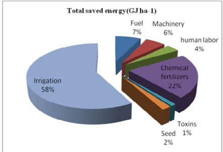
In Fig. 1 the shares of the various sources from total input energy saving are presented. Results revealed that

the highest contribution to the total saving energy was 58 % for Irrigation followed by chemical fertilizers (22 %)

and diesel fuel (7 %) energy inputs, respectively. Moreover the shares of machinery, human labor, Seed and Toxins

energy inputs were relatively low, indicating that they have been used in the right proportions by almost all the

farmers. Chauhan et al. (2006) reported that the contribution of fertilizer and diesel fuel energy inputs from total

saving energy in paddy production were 33% and 24%, respectively. Mousavi-Avval et al. (2011a) reported that the

contribution of electricity and seed energy inputs by 78.1% and 0.05% from total energy saving in soybean

production were the highest and lowest, respectively.

In the region, the high contribution of saving irrigation energy resulted from the low efficiency of ancient irrigation methods, which led to waste a lot of water and energy in the form energy. The high contribution of fertilizer energy inputs showed that all of farmers were not fully aware of proper time and quantity of fertilizers usage. Also nitrogen fertilizers were the main fertilizer in rice production which applied improperly in the rejoin. So, providing information to farmers and changing their incorrect behaviors can prevent loss of energy and also their harmful effects on environment. The high percent saving in diesel fuel shows the mismanagement in machinery employment in field operations.

FIGURE 1. Distribution of saving energy from different sources for rice production.

Improvements of energy indices

The improvements of energy indices for rice production are presented in Table 5. Energy use efficiency was calculated as 2.27 and 2.46, in present and target use of energy, respectively, showing an improvement of 7.46 %.

Also, energy productivity and net energy in target conditions were found to be 0.066 kg MJ

and 82.45 GJ ha

, respectively. The distribution of inputs used in the production of rice according to the direct, indirect, renewable and non-renewable energy groups are also given in Table 5. It is evident that by optimization of energy input, the shares of Indirect and non-renewable energy with respect to total energy input increased and also the shares of direct and renewable energy forms symmetrically decreased.

Mohammadi et al. (2011) reported by optimization of energy inputs in kiwifruit production the energy use efficiency by increasing of 13.86% can be improved to the value of 1.75. In another study, energy use efficiency for apple production was calculated as 1.16 and 1.31, in present and target use of energy, respectively, showing an improvement of 12.93% (Mousavi-Avval et al., 2011b).

TABLE 5

Improvement of energy indices for Rice production.

Items Unit Present quantity Optimum quantity Difference(%)

Energy use efficiency ratio 2.27 2.46 7.46

Energy productivity Kg MJ

0.061 0.066 7.46

Net energy gain GJ ha

77.88 82.45 5.54

Direct energy GJ ha

7.3 (11.92%) 6.8 (12.00%) -7.35

Indirect energy GJ ha

53.93 (88.08%) 49.86 (88.00%) -8.16

Renewable energy GJ ha

2.92 (4.77%) 2.66 (4.69%) -9.77

Non-renewable

energy GJ ha

58.31 (95.23%)

54 (95.31%) -7.98

Total energy input GJ ha

61.23 (100%) 56.66 (100%) -8.07

Setting realistic input levels for inefficient farmers

In Table 6 the pure technical efficiency (PTE), actual energy use and optimum energy requirement from different energy sources for individual inefficient farmers are shown. Also their average and standard deviation values are presented. Using this information, it is possible to advise a producer regarding the better operating practices by following his/her target energy requirement from different inputs to reduce the input energy levels to the target values while achieving the output level presently achieved by him. So, dissemination of these results will help to improve efficiency of farmers for rice production in the surveyed region. In the last column of Table 6 the ESTR percentage for 56 inefficient farmers are presented. As it can be seen, for inefficient farmers, ESTR ranges from under 1% (farmers no. 14, 31) to 15.99% (farmer no. 56), with the average of 9.47 %, indicating that between inefficient farmers, nos. 14, 31 were the best, and farmer no. 56 was the most inefficient one.

TABLE 6

The source wise actual and target energy use for inefficient farmers in the rice production (based on BCC model).

DMU PTE

Actual energy use (GJ ha⁻¹) Optimum energy requirement (GJ ha⁻¹) ESTR

(%)

Labour Machinery fuel Fertilizer Toxins irrigation seed Labour Machinery fuel Fertilizer Toxins irrigation seed

1 0.94 2.15 2.79 5.21 8.01 1.07 40.50 1.36 1.51 2.56 4.87 6.35 1.00 34.19 1.02 15.70

4 0.98 1.55 2.79 5.29 7.91 1.07 40.50 1.28 1.51 2.72 5.09 7.25 1.04 36.02 1.07 9.42

7 0.97 2.15 3.05 5.21 7.44 0.55 38.95 1.19 1.77 2.73 5.08 6.06 0.54 37.96 1.06 5.71

9 0.97 1.45 3.89 5.69 7.14 0.74 40.95 1.28 1.40 3.07 5.25 6.55 0.72 39.67 1.11 5.51

13 0.96 2.02 3.43 5.81 9.07 0.66 45.40 1.02 1.69 3.22 5.59 6.68 0.63 41.10 0.98 11.16

14 0.99 1.75 3.30 5.50 7.65 0.59 40.50 1.11 1.69 3.15 5.47 7.60 0.59 40.25 1.08 0.94

15 0.93 1.60 3.82 5.60 7.69 1.21 40.50 1.11 1.49 2.92 5.23 7.18 0.94 37.28 1.03 8.87

18 0.96 2.02 3.37 5.91 9.07 0.66 46.40 1.02 1.69 3.24 5.61 6.74 0.63 41.29 0.95 12.13

19 0.93 2.00 4.28 6.59 10.94 1.07 45.40 1.11 1.60 3.89 5.69 9.06 0.83 42.16 1.03 9.99

21 0.96 2.00 3.02 5.31 7.64 0.91 41.00 1.16 1.81 2.90 5.11 7.35 0.76 38.82 1.08 5.26

22 0.98 1.98 3.56 5.21 7.72 0.75 42.00 1.11 1.65 3.22 5.12 7.46 0.74 38.59 1.02 7.27

23 0.96 1.85 3.24 5.79 8.15 0.75 40.60 1.14 1.59 3.11 5.30 7.48 0.72 39.00 1.06 5.30

25 0.93 1.92 3.37 5.61 7.86 1.03 40.80 1.17 1.60 3.14 5.23 7.33 0.85 38.05 1.03 7.33

26 0.91 1.70 3.76 5.80 9.36 1.07 40.70 1.19 1.49 3.42 5.23 8.53 0.98 37.09 1.11 9.01

27 0.99 2.00 3.05 4.99 6.90 0.85 39.00 1.16 1.62 2.67 4.93 6.12 0.84 35.49 0.97 9.16

28 0.95 1.80 3.24 5.60 7.80 0.75 39.60 1.19 1.52 3.08 5.26 7.28 0.71 37.70 1.09 5.57

29 0.93 1.66 3.18 5.65 7.65 0.71 40.70 1.24 1.54 2.95 5.18 6.43 0.66 37.72 1.08 8.60

30 0.90 1.85 3.30 6.21 8.09 1.07 40.20 1.14 1.46 2.98 5.18 7.24 0.97 36.27 1.03 10.88

31 0.99 1.72 3.18 5.40 7.72 0.51 40.50 1.17 1.71 3.09 5.36 7.65 0.51 40.20 1.11 0.95

32 0.97 1.68 2.98 5.11 7.60 0.92 40.00 1.17 1.59 2.70 4.93 6.31 0.89 35.30 1.03 11.28

34 0.95 1.45 3.18 5.22 7.02 0.93 40.00 1.11 1.38 2.68 4.98 6.19 0.89 34.03 1.06 13.07

35 0.93 1.50 3.18 5.41 7.70 0.96 40.00 1.16 1.39 2.79 5.00 6.47 0.89 34.74 1.07 12.62

36 0.92 1.60 3.24 5.51 7.80 0.95 40.50 1.11 1.48 2.76 5.09 6.39 0.88 35.31 1.03 12.80

37 0.90 1.67 3.18 5.55 7.78 0.95 40.60 1.16 1.51 2.80 5.01 6.50 0.86 34.97 1.05 13.45

38 0.91 1.69 3.24 5.59 7.83 0.75 40.70 1.19 1.54 2.94 5.08 6.72 0.68 36.88 1.08 9.95

39 0.90 1.70 3.30 5.60 7.80 0.95 40.79 1.16 1.53 2.90 5.05 6.72 0.86 35.63 1.05 12.33

40 0.90 1.89 3.50 5.83 11.00 0.95 41.00 1.28 1.47 3.14 5.21 7.73 0.85 36.84 1.09 13.93

42 0.94 1.97 3.24 5.38 7.81 0.95 40.50 1.19 1.61 3.05 5.07 7.34 0.89 36.79 1.05 8.58

45 0.93 1.62 3.37 5.39 7.64 0.93 40.30 1.19 1.50 2.89 4.99 7.07 0.86 36.15 1.07 9.78

46 0.95 1.70 3.24 5.29 7.70 0.88 40.45 1.16 1.62 2.99 5.04 6.98 0.84 36.82 1.04 8.42

47 0.97 1.81 3.30 5.45 6.79 0.63 40.49 1.16 1.71 2.96 5.31 6.61 0.61 39.17 1.04 3.72

48 0.96 1.75 2.98 5.20 7.37 0.90 40.50 1.19 1.61 2.85 4.99 6.66 0.86 36.07 1.04 9.70

49 0.97 1.71 3.24 5.30 7.70 0.63 40.50 1.16 1.64 3.00 5.15 7.13 0.61 39.37 1.09 3.74

50 0.98 1.85 3.18 5.35 7.96 0.66 40.50 1.19 1.63 3.07 5.23 7.38 0.65 39.58 1.09 3.39

51 0.92 1.71 3.50 5.89 10.66 0.95 40.90 1.19 1.49 3.21 5.24 8.02 0.87 37.51 1.09 11.37

52 0.97 1.50 3.89 6.40 11.30 1.07 41.00 1.28 1.46 3.51 5.30 8.08 0.86 39.78 1.10 9.56

53 0.95 1.77 3.18 5.29 8.16 0.90 40.60 1.16 1.62 2.89 5.01 6.72 0.85 36.29 1.04 10.87

54 0.94 1.83 3.43 5.32 7.37 0.63 40.10 1.11 1.72 2.71 5.00 5.78 0.59 37.52 1.04 9.08

55 0.95 1.79 3.18 5.29 7.66 0.63 40.40 1.14 1.66 2.86 5.04 6.49 0.60 38.47 1.08 6.47

56 0.92 1.88 3.30 5.39 10.65 1.07 40.50 1.19 1.53 2.83 4.98 7.03 0.99 35.35 1.04 15.99

57 0.88 1.82 3.37 5.75 9.56 1.07 40.50 1.19 1.50 2.98 5.08 7.28 0.94 35.76 1.05 13.71

58 0.90 1.80 3.50 5.85 10.06 0.75 40.52 1.19 1.47 3.16 5.28 6.92 0.68 36.59 1.07 13.35

59 0.92 1.77 3.37 5.70 7.37 0.95 40.60 1.16 1.54 2.95 5.23 6.76 0.87 37.26 1.00 8.72

60 0.92 1.87 3.43 5.75 7.90 0.90 40.65 1.11 1.52 3.06 5.29 6.91 0.83 37.39 1.02 9.07

61 0.97 1.80 3.24 5.30 7.67 0.63 40.50 1.19 1.65 2.96 5.11 6.92 0.61 39.08 1.08 4.84

62 0.91 1.83 3.37 5.65 10.07 0.75 40.60 1.19 1.61 3.05 5.12 6.67 0.68 36.78 1.07 13.36

63 0.91 1.79 3.24 5.69 7.96 0.75 40.65 1.19 1.56 2.96 5.17 6.69 0.68 37.08 1.08 9.87

64 0.91 1.80 3.30 5.70 7.96 0.75 40.50 1.19 1.52 3.01 5.20 6.85 0.68 36.93 1.09 9.67

65 0.89 1.82 3.37 5.79 7.96 1.07 40.60 1.16 1.48 2.95 5.17 7.11 0.96 36.26 1.03 11.02

66 0.92 1.80 3.24 5.40 7.96 0.95 40.10 1.11 1.59 2.66 4.97 6.15 0.87 35.52 1.02 12.85

67 0.94 1.77 3.24 5.45 7.96 0.63 40.23 1.16 1.67 2.88 5.13 6.46 0.59 37.85 1.07 7.93

68 0.92 1.82 3.43 5.89 7.96 0.90 40.65 1.12 1.48 3.12 5.32 7.05 0.83 37.29 1.03 9.15

69 0.89 1.80 3.43 5.80 7.96 1.07 40.50 1.19 1.47 2.93 5.14 7.06 0.95 35.92 1.04 11.72

70 0.90 1.83 3.43 5.80 9.17 0.75 40.60 1.19 1.49 3.10 5.24 6.83 0.68 36.68 1.08 12.22

71 0.91 1.79 3.50 5.89 8.24 0.75 40.90 1.19 1.47 3.19 5.31 7.20 0.68 37.29 1.09 9.69

72 0.90 1.88 3.56 6.00 11.00 0.95 41.00 1.19 1.48 3.19 5.23 7.59 0.85 36.76 1.07 14.35

ave: 0.94 1.79 3.33 5.58 8.28 0.85 40.78 1.17 1.56 3.00 5.17 6.98 0.78 37.35 1.05 9.47

SD: 0.03 0.15 0.26 0.31 1.14 0.17 1.28 0.06 0.10 0.23 0.17 0.61 0.14 1.79 0.03 3.45

Conclusion

In this study, the non-parametric method of DEA was used to analyze the efficiencies of rice producers in Mazandaran province of Iran in energy points of view. Based on the results of the investigations, the following conclusions were drawn:

1. From the total of 72 farmers considered for the analysis, 9.7 % and 22.2 % were found to be technically and pure technically efficient, respectively.

2. The average values of technical, pure

technical and scale efficiency scores of farmers were

found to be 0.78, 0.95 and 0.82, respectively.

3. The energy saving target ratio for rice production was calculated as 7.47 % , indicating that by following the recommendations resulted from this study, about 4.57 GJ ha

of total input energy could be saved while holding the constant level of rice yield.

4. The irrigation energy had the highest potential for improvement by 58%, followed by chemical fertilizer and diesel fuel energy inputs.

5. The comparative results of energy indices revealed that by optimization of energy consumption, energy efficiency, energy productivity and net energy with respect to the actual energy use can be increased by 7.46 %, 7.46 % and 5.54 %, respectively.

6. It is suggested that new policies, such as providing information to farmers and using of modern methods of irrigation, are to be implemented to reduce the negative effects of energy inputs such as plant, soil and climate pollution.

References

1. Adler N, Friedman L, Sinuany-Stern Z. Review of ranking methods in the data envelopment analysis context. Eur J Oper Res 2002;140(2):249–65.

2. Angulo-Meza L, Lins MPE. Review of methods for increasing discrimination in Data Envelopment Analysis. Ann Oper Res 2002;116(1–4):225–42.

3. Anonymous. Annual agricultural statistics.

Ministry of Jihad-e-Agriculture of Iran.

http://www.maj.ir2010.

4. Avkiran NK. Investigating technical and scale efficiencies of Australian universities through data envelopment analysis. Socioecon Plann Sci 2001;35(1):57–80.

5. Bames A. Does multi-functionality affect technical efficiency? A non-parametric analysis of the Scottish dairy industry. J Environ Manage 2006;80(4):287–94.

6. Banker R, Charnes A, Cooper W. Some models for estimating technical and scale inefficiencies in data envelopment analysis. Manage Sci 1984;30:1078–92.

7. Boehmel C, Lewandowski I, Claupein W.

Comparing annual and perennial energy cropping systems with different management intensities. Agric Syst 2008;96(1–3):224–36.

8. Canakci A, Akinci I. Energy use pattern analyses of greenhouse vegetable production. Energy 2006;31:1243–56.

9. Cetin B, Vardar A. An economic analysis of energy requirements and input costs for tomato production in Turkey. Renew Energy 2008;33:428–33.

10. Cherati, F.E., H. Bahrami and A .Asakereh,.

Energy survey of mechanized and traditional

rice production system in Mazandaran Province of Iran. Afr. J. Agric. Res., 2011; 6(11), pp.

2565-2570.

11. Charnes A, Cooper WW, Rhodes E. Measuring the efficiency of decision-making units. Eur J Oper Res 1978;2:429–44.

12. Chauhan NS,Mohapatra PKJ, Pandey KP.

Improving energy productivity in paddy production through benchmarking—an application of data envelopment analysis.

Energy Convers Manage 2006;47(9–10):1063–

85.

13. Cooper W, Seiford LM, Tone K. Data envelopment analysis: a comprehensive text with models, applications, references and DEA-solver software. New York: Springer; 2007.

14. Erdal G, Esengun K, Erdal H, Gunduz O.

Energy use and economical analysis of sugar beet production in Tokat province of Turkey.

Energy 2007;32(1):35–41.

15. Fraser I, Cordina D. An application of Data Envelopment Analysis to irrigated dairy farms in Northern Victoria, Australia. Agric Syst 1999;59(3):267–82.

16. Galanopoulos K, Aggelopoulos S, Kamenidou I, Mattas K. Assessing the effects of managerial and production practices on the efficiency of commercial pig farming. Agric Syst 2006;88(2–

3):125–41.

17. Ginigaddara,G.A.S. and S.L.

Ranamukhaarachchi. Effect of conventional, SRI and modified water management on growth, yield and water productivity of direct-seeded and transplanted rice in central Thailand. Aust. J.

Crop Sci., 2009; 3(5): 278-286.

18. Hu JL, Kao CH. Efficient energy-saving targets for APEC economies. Energy Policy 2007;35(1):373–82.

19. IRRI,. A Handbook of Weed Control in Rice, International Rice Research Institute. Manila, Philippines, 2010.pp: 113.

20. Manes GS, Singh S. Optimal use of energy inputs for rice cultivation in Punjab. J Res PAU 2003;40(3-4):405.

21. Mikkola JH, Ahokas J. Indirect energy input of agricultural machinery in bioenergy production.

Renew Energy 2010;35:23–8.

22. Mobtaker HG, Keyhani A, Mohammadi A, Rafiee S, AkramA. Sensitivity analysis of energy inputs for barley production in Hamedan Province of Iran. Agric Ecosyst Environ 2010;137(3–4):367–72.

23. Mohammadi A, Omid M. Economical analysis

and relation between energy inputs and yield of

greenhouse cucumber production in Iran. Appl

Energy 2010;87(1):191–6.

24. Mohammadi A, Rafiee SH, Mohtasebi SS, Mousavi-Avval SH, Rafiee H. Energy efficiency improvement and input cost saving in kiwifruit production using Data Envelopment Analysis approach. Renew Energy 2011;36:2573–9.

25. Mousavi-Avval SH, Rafiee S, Jafari A,Mohammadi A. Optimization of energy consumption for soybean production using Data Envelopment Analysis (DEA) approach. Appl Energy 2011a;35:2156–64.

26. Mousavi-Avval SH, Rafiee S, Mohammadi A.

Optimization of energy consumption and input costs for apple production in Iran using data envelopment analysis. Energy 2011b;36:909–16.

27. Nassiri SM, Singh S. Study on energy use efficiency for paddy crop using data envelopment analysis (DEA) technique. Appl Energy 2009;86(7):1320–5.

28. Ozkan B, Fert C, Karadeniz CF. Energy and cost analysis for greenhouse and open-field grape production. Energy 2007;32(8):1500–4.

29. Rafiee S, Mousavi-Avval SH, Mohammadi A.

Modeling and sensitivity analysis of energy inputs for apple production in Iran. Energy 2010;35:3301–6.

30. Reddy AR, Sen C. Technical inefficiency in rice production and its relationship with farm- specific socio-economic characteristics. Ind J Agric Eco 2004;59(2):259.

31. Samadi-Maybodi, A. and E. Atashbozorg,.

Quantitative and qualitative studies of silica in different rice samples grown in north of Iran using UV-vis, XRD and IR spectroscopy techniques. Talanta, 2006; 70: 756-760.

32. SarIca K, Or I. Efficiency assessment of Turkish power plants using data envelopment analysis.

Energy 2007;32(8):1484–99.

33. Sexton TR, Silkman RH, Hogan AJ. Data envelopment analysis: critique and extensions.

In: Silkman RH, editor. Measuring efficiency: an assessment of data envelopment analysis. San Francisco: Jossey-Bass; 1986.

34. Sinha, S.K. and J. Talati,. Productivity impacts of the system of rice intensification (SRI): A case study in West Bengal, India. Agr. Water Manag 2007; 87: 55-60.

35. Singh S, Singh MP, Bakhshi P. Unit energy consumption for paddy–wheat rotation. Energy Convers Manage 1990;30:121.

36. Singh S, Singh S, Mittal JP, Pannu CJS, Bhangoo BS. Energy inputs and crop yield relationships for rice in Punjab. Energy – The Int J 1994;19:1061.

37. Singh S, Mittal JP, Verma SR. Energy requirements for production of major crops in India. Agric Mech Asia Afr Latin Am 1997;28(4):13.

38. Singh G. Optimization of energy inputs for crop production in Punjab. Unpublished Ph.D.

dissertation. Ludhiana, India: Department of Farm Power and Machinery, College of Agril.

Engg. Punjab Agricultural University; 2001.

39. Singh G, Singh S, Singh J. Optimization of energy inputs for wheat crop in Punjab. Energy Convers Manage 2004;45:453–65.

40. Unakitan G, Hurma H, Yilmaz F. An analysis of energy use efficiency of canola production in Turkey. Energy 2010;35:3623–7.

41. Zangeneh M, Omid M, Akram A. A comparative study on energy use and cost analysis of potato production under different farming technologies in Hamadan province of Iran. Energy 2010;35:2927–33.

42. Zhang X, Huang GH, Lin Q, Yu H. Petroleum- contaminated groundwater remediation systems design: a data envelopment analysis based approach. Expert Syst Appl 2009;36(3, Part 1):5666–72.

43. Zhou P, Ang BW, Poh KL. A survey of data envelopment analysis in energy an environmental studies. Eur J Oper Res 2008;189:1-18.

6/17/2013