九州大学学術情報リポジトリ
Kyushu University Institutional Repository
医療応用のための磁気ナノ粒子イメージング法の開 発
ヌルミザ, ビンティ, オスマン
https://doi.org/10.15017/1441260
出版情報:Kyushu University, 2013, 博士(学術), 課程博士 バージョン:
権利関係:Fulltext available.
i
Magnetic Nanoparticle Imaging for Biomedical Applications
Nurmiza Binti Othman
ii
Magnetic Nanoparticle Imaging for Biomedical Applications
by
Nurmiza Binti Othman
D
OCTORALT
HESISS
UBMITTED TO THEG
RADUATES
CHOOL OFI
NFORMATIONS
CIENCE ANDE
LECTRICALE
NGINEERING IN PARTIAL FULFILLMENT OF THE REQUIREMENTS FOR THE DEGREE[
DOCTOR OF PHILOSOPHY]
(D
EPARTMENT OFE
LECTRICAL ANDE
LECTRONICE
NGINEERING)
KYUSHU UNIVERSITY Fukuoka, JAPAN
Supervisor: Professor Dr. Keiji Enpuku
March 2014
© Nurmiza Binti Othman 2014
__________________________________________________
iii
List of Contents
List of Contents iii
List of Tables v
List of Figures vi
List of Parameters x
Chapter One: INTRODUCTION
1.1 Background 1
1.2 Possibilities in Imaging Using the MNPs 3
1.2.1 Detection Methods of MNPs 3
1.2.2 Basic Concepts of MPI 4
1.3 MPI for Sentinel Lymph Node Biopsy 9
1.3.1 Sentinel Lymph Node Biopsy 9
1.3.2 Principle and Technique 10
1.3.3 MNP Imaging for SLNB 11
1.4 Aims of Research 13
1.5 Thesis Outline 14
References 15
CHAPTER TWO: MAGNETIC NANOPARTICLES (MNPs)
Introduction 18
2.1 Magnetic Nanoparticles 18
2.1.1 Magnetism and Magnetic Material 18
2.1.2 Superparamagnetic Iron Oxide Nanoparticles (SPIONs) 19
2.2 Nonlinear Magnetization of MNPs 26
2.2.1 Magnetic relaxation 26
2.2.1.1 Brownian Relaxation 26
2.2.1.2 Neel Relaxation 26
2.2.2 Harmonic Signals 27
2.3 Applications in the Biomedical Field 28
2.3.1 Drug delivery 30
2.3.2 Hyperthermia 32
2.3.3 Immunoassay 34
2.3.4 Magnetic Particle Imaging (MPI) 35
References 36
CHAPTER THREE: CHARACTERIZATION OF MNP SAMPLES FOR MPI
3.1 Introduction 37
3.2 MNP Sample Preparation 39
3.3 Harmonic Signal Measurement 40
3.3.1 Measurement Method 40
3.3.2 Measurement Result: Harmonic Spectrum 41
3.4 Harmonic Signal Analysis 42
3.4.1 M-H Curve Measurement 42
3.4.2 AC Susceptibility Measurement 44
3.4.3 m-EB Relationship 47
3.4.4 Conditions of Observing Rich Harmonic Spectrum for MPI 47 3.4.5 Fraction of MNPs That Contribute to Harmonic Signals 48 3.5 Numerical Simulation: Landau-Lifshitz-Gilbert (LLG) Equation 49 3.6 Comparison: Experimental and Numerical Simulation Results 51
3.7 Discussion 52
3.8 Conclusions 52
References 52
iv CHAPTER FOUR: MNP IMAGING SYSTEM DEVELOPMENT USING THE
SECOND HARMONIC DETECTION
4.1 Introduction 54
4.2 Harmonic Component Analysis 55
4.2.1 Measurement Setup 56
4.2.2 Measurement Result 58
4.2.3 Discussion: Comparison of V2p/V1p and V2p/V3p 58 4.2.4 HDC and HAC Relationship for Obtaining Second Harmonic Signal Peak 59
4.2.5 Discussion 60
4.3 Magnetization Method of MNPs 60
4.4 Second Harmonic Detection-based MNP Imaging System 62
4.4.1 MNP Sample 62
4.4.2 Measurement System 63
4.4.3 Excitation Coil 66
4.4.4 Pickup Coil 69
4.5 Resonant Circuit 71
4.5.1 Resonant Circuit for Excitation Circuit 71
4.5.2 Resonant Circuit for Detection Circuit 74
4.6 System noise 75
4.6.1 Thermal Noise 76
4.6.2 Lock-in Amplifier Input Noise 76
4.6.3 Total System Noise 76
4.7 Conclusions 78
References 78
CHAPTER FIVE: SENSITIVITY AND SPATIAL RESOLUTION OF MNP IMAGING
5.1 Position identification from Bz measurement 79
5.1.1 Sensitivity of the Measurement System 80
5.1.2 Position Identification in xy Plane (One MNP Sample) 80 5.1.3 Position Identification in xy Plane (Two MNP Samples) 82 5.1.4 Comparison: Experimental and Numerical Simulation Result 85 5.2 Signal Processing for High Spatial Resolution Image 88
5.2.1 Singular Value Decomposition (SVD) 88
5.2.2 MNP Density Distribution in xy Plane 90
5.3 Detection of Two MNP samples With Different Weights of Fe 92
5.4 Depth Estimation from Bz Measurement 94
5.4.1 Depth and Magnetic Field Relationship 95
5.4.2 Depth Estimation of Two MNP Samples from Bz Measurement 96
5.5 Depth Estimation from Bxy measurement 98
5.5.1 Depth and Magnetic Field Relationship 98
5.5.2 Depth Estimation of Two MNP Samples from Bxy Measurement 100
5.6 SVD Analysis with Error in Depth Information 104
5.7 Towards Better Imaging 106
5.7.1 Immobilization Method 106
5.7.2 New MNPs with High Nonlinearity 107
5.7.3 MNP Imaging Using New MNP 108
5.7.3.1 Position Estimation in xyz Plane 108
5.7.3.2 Depth Estimation 112
5.8 Conclusions 112
References 113
CHAPTER SIX: CONCLUSIONS AND FUTURE WORK
6.1 Conclusions and Contribution 114
6.2 Future Work 115
ACKNOWLEDGEMENTS 117
v
L IST OF TABLES
Table 1.1 : Overview of MPI Scanners. 8
Table 3.1 : Specifications of Prepared MNP Samples. 39
vi
L IST OF FIGURES
Figure 1.1 : Signal generation in MPI. (a) Normal response of MNPs to an externally applied oscillating field, and (b) saturated response of MNPs when a static field is superimposed on the oscillating field. 4 Figure 1.2 : A strong magnetic field gradient forms a zero magnetic field point
known as FFP. 7
Figure 1.3 : Examples of MPI scanner (a) cave-shaped scanner with a cylindrical bore, and (b) single-sided scanner. 7 Figure 1.4 : Lymphatic system draining the breast, indicating tumor and
sentinel lymph node. 10
Figure 1.5 : Sentinel Lymph Node Biopsy. 11
Figure 1.6 : Non-cryogenic SentiMagTM, commercially available in CE-mark
accepted countries. 13
Figure 2.1 : Magnetic behavior of different materials: FM is ferromagnetic, SPM is superparamagnetic, and PM is paramagnetic material. 19 Figure 2.2 : Structure of magnetic domain and domain wall. 23 Figure 2.3 : Illustration of the variables used to model magnetic fluctuation in
ferromagnetic material. 23
Figure 2.4 : An illustration of a 180 ° domain wall. 23
Figure 2.5 : Magnetic domain in magnetic material (a) multi-domain, and (b)
single domain. 24
Figure 2.6 : Concept of superparamagnetic material. 24
Figure 2.7 : The randomization of magnetization which takes place by
excitation field H over EB. 25
Figure 2.8 : The Langevin function to demonstrate the relative magnetization of a non-interacting and freely rotable magnetic moments system. 25 Figure 2.9 : Model of the (a) Brownian-relaxation-dominated and (b) Neel-
relaxation-dominated magnetic marker. 27
Figure 2.10 : (a) Schematic drawing and (b) an image of a spherical MNP consists of a magnetic core with biocompatible coating for
biomedical applications. 30
Figure 2.11 : A hypothetical magnetic drug delivery system shown in cross- section: a magnet is placed outside the body so that its magnetic field gradient might capture magnetic carriers flowing in the
circulatory system. 32
Figure 2.12 : Magnetic hyperthermia. 33
Figure 2.13 : Principle of magnetic immunoassay detected by a SQUID
magnetometer. 35
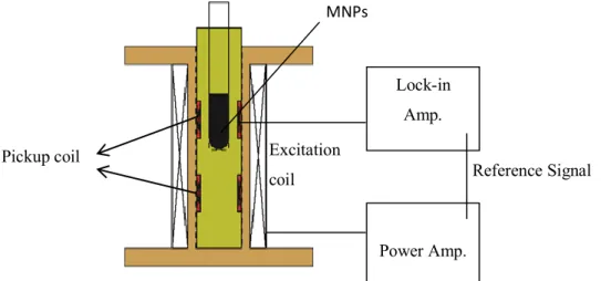
Figure 3.1 : Schematic drawing of a spherical MNP consisting of a magnetic core composed of elementary and agglomerate particles. 39 Figure 3.2 : Schematic drawing of an experimental setup for harmonic signal
measurement. 40
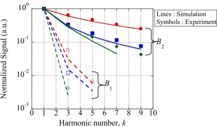
Figure 3.3 : Closed-up image of the experimental set up shown in Fig. 3.2. 41 Figure 3.4 : Harmonic spectra of Resovist, fluidMAG, and SupraBead MNPs
under B1 and B2 excitation. 41
Figure 3.5 : Comparison of normalized signals between measurement and
numerical simulation results. 42
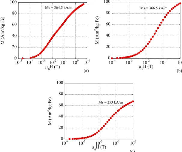
Figure 3.6 : M-H curve of suspended samples of (a) Resovist, (b) fluidMAG,
and (c) SupraBead MNPs. 43
Figure 3.7 : m distribution of suspended samples of (a) Resovist, (b)
fluidMAG, and (c) SupraBead MNPs. 44
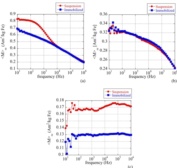
Figure 3.8 : Frequency dependence of real magnetization of immobilized and suspended samples of (a) Resovist, (b) fluidMAG, and (c)
SupraBead MNPs. 46
Figure 3.9 : σ distribution of (a) Resovist and (b) fluidMAG MNPs. 46 Figure 3.10 : m-σ relationship of (a) Resovist and (b) fluidMAG MNPs.
vii Double arrow symbols indicate the fraction of MNPs that contributes to the harmonic signals at B1 = 1.4 mT and B2 = 28
mT. 47
Figure 3.11 : Distribution of magnetic moment m within MNPs. Double arrow symbols indicate the fraction of MNPs that contributes to the
harmonic signals at B2 = 28 mT. 49
Figure 3.12 : Illustration of the easy axis unit vector and magnetic moment
vector. 50
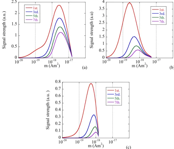
Figure 3.13 : Harmonic signal strength generated by each m distributed in (a) Resovist, (b) fluidMAG, and (c) SupraBead MNPs. Harmonic
signals with k=1 to 7 are shown. 51
Figure 4.1 : Harmonic signal measurement with an immobilized Resovist
sample. 57
Figure 4.2 : Dependence of harmonic signal amplitude on HDC when the rms value of μ0HAC fields were fixed at (a) 0.5, (b) 1.0, (c) 2.5, and (d) 5.0 mT. HDC was varied between μ0HDC = 0–5 mT. 57 Figure 4.3 : Ratio of the peak value of the second harmonic component V2p to
that of the (a) fundamental component V1p and (b) third
component V3p, for varying HAC. 59
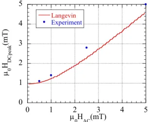
Figure 4.4 : Relationship between HDCP and HAC when the peak value of the
second harmonic signal was obtained. 60
Figure 4.5 : Schematic diagram of applying Bm in perpendicular with the
pickup coil. 61
Figure 4.6 : Schematic diagram of applying Bm in parallel with the pickup
coil. 62
Figure 4.7 : An image of immobilized Resovist placed into a cell with a
diameter of 6 mm and a height of 5 mm. 63
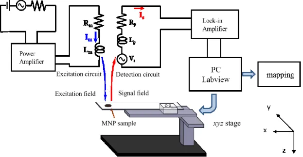
Figure 4.8 : Signal chain of the MNP detection system. 64 Figure 4.9 : Schematic of the MNP detection system. The inset shows its real
image. 64
Figure 4.10 : Physical arrangement of excitation coil and pickup coil of (a) Bz
and (b) Bx and By measurement, together with the MNPs position. 65 Figure 4.11 : Example of the measured signal of (a) vertical and (b) horizontal
component of Bs2. 66
Figure 4.12 : Single-layer circular coil. 68
Figure 4.13 : Schematic diagram of the multilayer excitation coil. 68 Figure 4.14 : Magnitude of the magnetic field according to the MNPs sample
with respect to the distance from the pickup coil, z. 69 Figure 4.15 : Real image of pickup coil of (a) Bz and (b) Bx and By
measurement. 70
Figure 4.16 : Resonant circuit. 71
Figure 4.17 : DC current bypass circuit with LC series resonant circuit. 73 Figure 4.18 : Current path at resonance for the case of (a) AC and (b) DC
current. 73
Figure 4.19 : Resonant circuit for the readout of pickup coil. 74 Figure 5.1 : Schematic of the MNP detection system. The inset shows its real
image. 79
Figure 5.2 : Relationship between the detected signal and the depth z. 100 μg
of MNP sample was used. 80
Figure 5.3 : (a) Contour map of Bz signal detected from one MNP sample, and (b) waveform of Vz along the x-axis at y = 0. The 100-μg MNP sample was located at z = 20 mm under the pickup coil. 81 Figure 5.4 : (a) Contour map of Bz signal detected from one MNP sample, and
(b) waveform of Vz along the x-axis at y = 0. The 100-μg MNP sample was located at z = 30 mm under the pickup coil. 82 Figure 5.5 : Two MNP samples with 100 μg Fe were placed into cells with
diameter of 6 mm and were separated by Δx. 83
viii Figure 5.6 : Contour map of Bz signal detected from two MNP samples of
similar weight (100 μg) were located at (a) z = 10 mm, (b) z = 15 mm, (c) z = 20 mm, (d) z = 25 mm, and (e) z = 30 mm under the pickup coil and were separated by Δx = 20 mm. 84 Figure 5.7 : The corresponding waveform of Vz along the x-axis at y = 0 for
MNP samples used in the each case as shown in Fig. 5.6. 85 Figure 5.8 : Reciprocity theoerem of voltage signal induction at the pickup
coil. 86
Figure 5.9 : Simulation result of the contour map of the Bz signal for the case of (a) one MNP sample located at z = 20, and (b) two MNP samples were located at z = 20 mm and were separated by Δx =
20 mm. 87
Figure 5.10 : Waveform of the Bz signal along the x-axis at y=0 for the case of (a) one MNP sample located at z = 20, and (b) two MNP samples were located at z = 20 mm and were separated by Δx = 20 mm.
Solid and dashed lines represent the numerical simulation and
experimental result, respectively. 88
Figure 5.11 : Principle of the SVD analysis. 90
Figure 5.12 : MNP density distribution n(x,y) obtained via SVD analysis. Two MNP samples of similar weight (100 μg) were located at (a) z = 20 mm and (b) z = 30 mm below the detection coil, and were
separated by Δx = 20 mm. 91
Figure 5.13 : Bz (red line) and MNP distribution n (blue line) along the x axis at y = 0 for two MNP samples located at (a) z = 20 mm and were
separated by Δx = 20 mm. 92
Figure 5.14 : Two MNP samples with different weights (100 μg and 50 μg of
Fe) were separated by Δx. 92
Figure 5.15 : Contour map of Bz signal detection. Two MNP samples with different weights (100 μg and 50 μg) were located at z = 20 mm
and were separated by Δx = 20 mm. 93
Figure 5.16 : (a) MNP density distribution n (x, y) obtained via SVD analysis using Bz signal detection. (b) Bz (red line) and MNP distribution n (blue line) along the x axis at y = 0. Two MNP samples with different weights (100 μg and 50 μg) were located at z = 20 mm
and were separated by Δx = 20 mm. 94
Figure 5.17 : Magnetic field generated at a point P(x,y,z) by a point-like MNP sample having a magnetic moment mz in the z-axis. 96 Figure 5.18 : An example of the distribution of Bz (red line) and dBz/dx (blue
line) along the x axis at y = 0 of one MNP sample located at z =
20 mm. 96
Figure 5.19 : Distribution of the derivative of Bs2 detected in z axis with respect to xy plane of two MNP samples having similar weight, located at (a) z = 15, and (b) z = 20 mm, and were separated by Δx = 20 mm. 97 Figure 5.20 : Contour map of the field (a) Bx and (b) the distribution of Bx
along the x axis at y = 0 from one MNP sample located at z = 20
mm. 99
Figure 5.21 : Relationship of depth and width of the peak value of one MNP
sample. 100
Figure 5.22 : Detection of Bs2 in horizontal component of (a) Bx and (b) By. 101 Figure 5.23 : Contour map of the field (a) Bx and (b) By together with their
respective distribution of Bx along the x axis at y = 0 when two MNP samples of similar weight (100 μg) were separated by Δx =
20 mm and located at z = 20 mm. 101
Figure 5.24 : Contour map of the field Bxy when two MNP samples of similar weight (100 μg) were separated by Δx = 20 mm and located at z =
20 mm. 102
Figure 5.25 : (a) αy vs. z and (b) αx - αy vs. Δx. The results were obtained from
ix
the Bxy contour map shown in Fig. 5.24. 103
Figure 5.26 : MNP density distribution n(x,y) obtained via SVD analysis of two MNP samples of similar weight (100 μg) were located at z = 20 mm with Δx = 20 mm when (a) z’=15 mm, (b) z’=21.1 mm, and
(c) z’=25 mm. 105
Figure 5.27 : MNP distribution n along the x-axis at y = 0 and z = 20 ± 5 mm.
Two MNP samples of similar weight (100 μg) were located at z =
20 mm with Δx = 20 mm. 106
Figure 5.28 : Resovist sample immobilized with (a) gypsum coagulant and (b)
glycerol. 107
Figure 5.29 : Magnitude of the harmonic signals of Resovist prepared in
glycerol and gypsum. 107
Figure 5.30 : Comparison of the magnitude of the second harmonic component
of MS1 and Resovist. 108
Figure 5.31 : Magnetic field map of each MNP sample located at the 30mm depth. (a) Resovist_gypsum, (b) Resovist_glycerol, and (c)
MS1_glycerol. 110
Figure 5.32 : Comparison of the waveform of Vz at the centerline of each
sample located at the 30mm depth. 111
Figure 5.33 : MNP density distribution n(x,y) obtained via SVD analysis. Two MS1 samples of similar weight (100 μg) were located at z = 30 mm below the pickup coil and were separated by Δx = 20 mm. 111
Figure 5.34 : Depth specification of MS1 sample. 112
x
LIST OF PARAMETERS
H (A/m) : Applied magnetic field Ms (A/m) : Saturation magnetization
m (Am2) : Magnetic moment per single marker M (Am2/kg Fe) : Magnetic moment per 1 kg Fe L(ξ)=coth(ξ)-1/ξ : Langevin function
T k mH/ B μ
ξ 0 : Parameter for Langevin function EB (J) : Anisotropy energy
σ= EB/kBT : Normalized energy τN=τoexp(EB/kBT) : Neel relaxation time
τo (s) : Characteristic time of Neel relaxation kB (J/K) : Boltzmann constant
T (K) : Absolute temperature
SV (V2/Hz) : Power spectrum of voltage noise Q : Quality factor of resonant circuit
1
Chapter 1 INTRODUCTION
1.1 BackgroundMagnetic nanoparticle (MNP) is a class of nanometer-scaled particle whose magnetic properties can be easily controlled and manipulated using externally applied magnetic field. Below approximately 30 nm in diameter, it exhibits superparamagnetic behavior as a response to an externally applied magnetic field, having a high saturation magnetization without any hysteresis in zero field excitation. Commonly consisted of magnetic elements based on metals, namely, iron, nickel and cobalt or metal oxides, MNP has been involved in different ways in the development of modern technologies. For instance, MNP plays important roles in many devices such as motors, generators, sensors, and hard disks [1].
In addition, MNP has also become the focus of much research recently due to its special physical properties, non-toxicity, and its ability to function at the cellular and molecular level of biological interactions. These show the potential use in biomedical field applications. Polymer-coated MNP is usually known as magnetic marker or tracer. Thus far, carboxyl-dextran-coated formulated iron oxide MNPs have been used as contrast agents to enhance the visibility of internal body structures of living organism during the magnetic resonance imaging (MRI). Therefore, such clinical applications of magnetic immunoassay, drug delivery, hyperthermia, and last but not least magnetic particle imaging (MPI) can be seriously considered in the near future [2]-[3].
Worldwide many working groups showed the feasibility to image molecules in vivo by introducing various scanning modalities that contribute to medical imaging. In medical imaging, parts of the human body are imaged to reveal, diagnose, or examine disease clinically. It is also used in medical science such as the study of normal anatomy and physiology. Along with advances in imaging technologies such as MRI, interventional computed tomography (CT), and fluoroscopy including intra-arterial digital subtraction angiography, MPI as a novel imaging technology can promise excellent imaging properties of high spatial and temporal resolution, high sensitivity without ionizing radiation.
The basic principle of MPI was firstly introduced by B. Gleich and J. Weizenecker in 2005 [4].
MPI quantitatively measures the spatial distribution of MNPs used as tracers injected into human body. The system employs the nonlinear magnetization characteristic of the MNPs under large excitation field which generates signal consists of fundamental excitation frequency as well as of harmonics. For spatial encoding, the principles of Field Free Point (FFP), Field Free Line (FFL) and Field of View (FOV) are introduced to obtain high resolution image.
2 The standard MPI system introduced in earlier stages was set up as a cave-shaped system where imaging take places when MNPs be recorded at the FOV lies in between a symmetric coil configuration [4]. However, the size of specimens to be fixed into the FOV area is limited due to the limited size of the cave itself. In 2009, T. F. Sattel et al. introduced a single-sided MPI scanner where imaging of specimen of interest simply can be done just from one side [5]. Hence, the problem of the specimen fitting into the cave-shaped scanner no longer exists.
For in vivo application of MNP imaging, MPI shows possibilities in 3D real-time imaging of cardio- and neuro-vascular, stem cell-tracking, and also of sentinel lymph node biopsy (SLNB) for the diagnosis and treatment of breast cancer. For example, recently, Weizenecker et al. successfully revealed the first in vivo result of 3D real-time imaging structures of a beating mouse heart that have been obtained via the MPI system [6].
MNPs injected into human body are generally collected by cells of mononuclear phagocyte system, and then carried to lymph nodes at where they accumulated for a certain time period. This characteristic can be employed in lymph node assessment for breast cancer staging, in which breast cancer is known as the second leading cause of cancer death in women after the cervical cancer.
SLNB is a more gentle method for assessment of lymphatic system opposed to currently used methods of radical axillary lymph node dissection, mammograms of breasts, CT scan, MRI, and/or positron emission tomography (PET) scans.
MNPs used as tracer is injected into the tumor area. It flows through the lymph vessel to reach the sentinel lymph node (SLN) and allows the specific localization by using a detection system of MPI [7]. Here, SLN is defined as the first lymph node at which cancer cells appear before spreading to other lymph nodes. In SLNB, the SLN is incised by the pathologist to check either cancer cells are already spread to the area or not.
Thus far, previous high-sensitivity MNP imaging systems have been developed on the basis on various detection methods employing the three types of measurement as follow. Firstly, AC susceptibility measurement of MNP by applying a weak excitation field to the MNPs and the resulting signal is detected [8]-[10]. The second type is magneto-relaxometry signal of MNPs measurement by detecting the relaxation signal after an external applied field is switched off [11]- [12]. Finally, harmonic signals measurement generated from the nonlinearity of the M-H curve of MNPs under strong excitation field [4]-[6]. Numerous studies have been performed in order to improve the detection system performance and achieve high temporal and spatial resolution imaging system.
3
1.2 Possibilities in Imaging Using the MNPs
1.2.1 Detection Method of MNPs
MNPs show possibilities to be used for in vivo diagnostics in medical imaging. In this application, MNPs are injected in human body and are detected at the body surface after being magnetized. However, since MNPs possess a dipolar magnetic field, the signal decays very rapidly with the distance between the MNPs and the detection sensor. Therefore, a highly sensitive system is needed for MNP detection.
Thus far, three methods have been introduced to detect MNPs especially for in vivo applications:
AC susceptibility, magnetorelaxometry, and harmonic signal detection. First of all, for a system based on the AC susceptibility measurement, the linear region of the M-H curve of MNPs is used. A weak excitation field is applied, and the resulting signal field from the MNPs is detected [8]-[10].
The advantage of using this method is that excitation device can be easily miniaturized due to small field need for excitation. However, since the signal field has similar frequency with the excitation field, and the amplitude is much smaller than the excitation field, hence, it is crucial to decrease the interference of the excitation field and a stable detection system is difficult to be obtained.
The second method to detect MNPs is known as magnetorelaxometry. In this technique, magnetic field relaxation of MNPs is detected after an external field, e.g. pulse magnetic field is turned off. The relaxation time is strongly influenced by the size of the MNPs if they are bound to surfaces. The size dependence follows approximately the exponential of the volume of the particle and thus the relaxation time changes rapidly with particle diameter. Moreover, since there is no magnetic field excitation during the signal relaxation, significant problem of interference from the excitation field in AC susceptibility method can be avoided [11]-[13]. Magnetic relaxation begins from the moment the external field is turned off. Therefore, it is important to make short the time to turn off the excitation field and the time to start measuring magnetic relaxation after the excitation field has been turned off.
The third method uses the nonlinear response of the M-H curve for detecting a harmonic signal from MNPs. In this method, a modulating magnetic field is applied and increased to a certain level at which the nonlinear response occurs and generates harmonic signals. Since harmonic signals have different frequencies with the excitation frequency, interference from the excitation field can be significantly decreased, and sensitivity can be improved [4]-[6]. Magnetic particle imaging (MPI) is a representative method that uses harmonic signals and will be introduced in the next section.
4
(a) (b) Fig. 1.1: Signal generation in MPI. (a) Normal response of MNPs to an externally applied oscillating field, and (b) saturated response of MNPs when a static field is superimposed on the
oscillating field.
1.2.2 Basic Concepts of MPI
Over the past decade, possibilities of MPI as new medical imaging technique have captured the interest of many researchers worldwide. The history dates back to 2005 where B. Gleich and J.
Weizenecker introduced the principle of MPI as a tomographic imaging method that can quantitatively measure the spatial distribution of a MNPs tracer [4].
Figure 1.1(a) shows the signal generation in MPI. MNPs which are subjected to an oscillating field will react with a nonlinear magnetization response as described by the Langevin function. The nonlinearity of the MNPs magnetization will produce signal consists of the fundamental excitation frequency as well as of harmonics that can be measured with an appropriate pickup coil arrangement.
The concentration of the MNPs can be reconstructed quantitatively based on the harmonics, once the fundamental signal is separated.
In the proposed basic principle of MPI, MNPs tracer is injected to, or is administred into, the sample to be measured. The sample then is placed in a static selection field (also known as gradient field), and an oscillating magnetic field is superimposed. Finally the sample is moved to discrete positions and the magnitudes of the harmonics are recorded for spatial encoding. An image of the magnetic tracer in the sample is directly obtained by mapping the magnitude of the harmonics. Since its introduction in 2005, MPI has undergone much development especially in terms of hardware evolution, MNPs design and optimization of image reconstruction methods.
For spatial encoding, the principles of Field Free Point (FFP), Field Free Line (FFL) and Field of View (FOV) are introduced to obtain high spatial resolution image. Normally, two magnets are arranged in Maxwell configuration, to generate a gradient field that exhibits a symmetric point with a zero magnetic field, referred as the FFP (Fig. 1.2). Figure 1.1(b) shows that MNPs have a
5 saturated magnetization when a static field is superimposed on the oscillating field. Therefore, within the FFP, MNPs’ magnetization is free to follow the excitation field to produce MPI signal.
Otherwise, the magnetization becomes saturated when MNPs are outside of the FFP, and are unable to respond to the applied modulating field. Hence, MPI signal is not produced anymore. For currently available MNPs and 6T/m gradients, the FFP is in a few millimeter scale spheroid.
Next, there are two fundamental ways to acquire image that represents the quantitative distribution of the MNPs tracer. The first method is by mechanical movement of MNPs tracer around the FFP or FFL. The second method is field-induced movement of FFP or FFL. In this case, they are moved electrically through the FOV by using a time-varying, homogenous magnetic field, named drive field.
Although MPI is still new when compared to other imaging tools, various scanners with different coil topologies and geometrics as well as imaging concepts have already been developed (Table 1.1).
The standard MPI scanner introduced in the earlier stages of MPI was set up as a cave-shaped system where imaging process takes place when MNPs be recorded at the FOV lies in between a symmetric coil configuration. Images are reconstructed using the frequency domain. While showing good field quality in terms of field homogeneity and gradient linearity, however, the size of specimens to be fixed into the FOV area is limited due to the limited size of the cave itself.
In 2009, T. F. Sattel et al. introduced a single-sided MPI scanner where the imaging of specimen of interest simply can be done just from one side [5]. Large patient sizes and full patient access are permitted. Hence, the problem of the specimen fitting into the cave-shaped scanner no longer exists.
However, this kind of coil topology shows a strongly inhomogeneous spatial resolution, which decreases with increasing distance to the scanner. Both concepts are shown in Fig. 1.3.
MPI allows measuring the change of particle magnetization as a voltage signal at particular pickup coil. MPI image can be obtained by reconstructing the spatial distribution of the MNPs. For this purpose, several approaches have been introduced thus far: harmonic space MPI, x-space MPI, FFL based MPI, and narrowband MPI.
The earliest image reconstruction method is known as harmonic space MPI [4]-[6]. It relies on a system matrix to pre-characterize the signal response of MNPs. A system matrix is generated by placing a delta sample of the MNPs tracer at each position of the FOV and measuring the corresponding frequency spectrum. It is also either can be modeled according to the particle characteristics and the scanner properties.
For image reconstruction using this technique, it is necessary to find the MNP response for each harmonic signal detected. A linear system of equation formed by a system matrixSˆ linking the unknown spatially dependent MNPs tracer concentration cˆ and the received Fourier transformed voltage signaluˆ can be expressed as
6
u c
Sˆ ˆ. (1.1)
System matrix gives the connection between the spatially distributed MNPs and the corresponding measured Fourier transformed voltage signal. Calculation of the MNPs tracer concentration then can be solved as
u S
cˆ ˆ1ˆ. (1.2)
Once the system matrix is measured, reconstruction is achieved through matrix inversion techniques such as singular value decomposition and algebraic reconstruction. The disadvantage of using the harmonic space method is that the matrix inversion can be quite complex and ill-posed, since the system matrix is large and contains more than billion elements. Information on the inversion technique are summarized elsewhere [14]-[16].
Beyond the computational challenges, another challenge is robustness. If the pre-characterization scans do not accurately reflect the tracer’s in vivo micro-environment, then the reconstructed image may have artifacts. For example, system matrix is usually acquired in water, which has a different viscosity than blood. These variations could produce modeling errors and lead to a less accurate system matrix, which would translate to imaging artifacts.
Alternatively, the reconstruction can be performed in the time domain using the x-space theory as introduced by P. W. Goodwill et al. [17]. Under the assumption of homogenous magnetic fields, i.e.
assuming a linear shift-invariant system, and based on the Langevin theory of superparamagnetism, a correlation between FFP position and induced voltage signal can be established and a direct reconstruction becomes possible. The native MPI image is expressed as a convolution of the MNPs distribution with the point spread function (PSF) of the system.
Mathematically, x-space theory describes MPI process in 1D (magnetization changes in x axis).
The raw MPI signal can be expressed as
x
tH x G
h x m dt B
B d t
s s
sat t x x s
φ ρ
1
1 (1.3)
where dt
dφ is the changes of flux-converted magnetization,ρ
x is the MNPs distribution, xs
t is the instantaneous position of the FFP, and xs
t is the instantaneous velocity of the FFP in the FOV.Besides that, several parameters also control the magnitude of the received signal, including the sensitivity of the pickup coil B1, the magnetic moment of the MNPs m, the gradient strength G, and the field sufficient for saturation of the MNPs, Hsat.
It has been shown that the magnetization of MNPs is nonlinear and obeying the Langevin function. As the voltage induction in pickup coil is based on the detection of the change in the magnetization level of the MNPs, hence, the point spread function (PSF) in 1D is expressed as the
7 derivative of the Langevin function L
and has the simple form of
Hsat
L Gx x
h
(1.4)
which resembles to a Lorentzian function. It has a full-width-half-magnitude (FWHM) that becomes finer with increasing gradient G and decreasing Hsat.
The raw MPI signal s
t is converted into x-space MPI image ρ
x using a simple two-step process of (1) velocity compensation followed by (2) gridding of the received signal to the instantaneous position of FFP. As MPI signal is simply a sampling of the native MPI image at the instantaneous position of the FFP, then, by knowing the position and velocity of the FFP through the FOV, a native MPI image can be reconstructed. The resulting image can be shown as
t x h xx t s G mB t H x
s
sat
ρ
ρ
1
. (1.5)
Fig. 1.2: A strong magnetic field gradient forms a zero magnetic field point known as FFP.
(a) (b)
Fig. 1.3: Examples of MPI scanner (a) cave-shaped scanner with a cylindrical bore, and (b) single-sided scanner.
8 Table 1.1: Overview of MPI Scanners [14].
The most significant advantage offered by x-space MPI over harmonic space MPI is that no matrix inversion or pre-characterization is required. In addition, no modeling regarding the in vivo micro-environment is required. Therefore, robust and real-time image reconstruction can be obtained.
A summarized overview of this theory has been reported elsewhere [18].
Besides FFP imaging, an alternative coil arrangement to generate FFL was introduced by Weizenecker et al. [19]. A projection image can be produced with higher sensitivity due to the integral of MNPs contributed along the FFL. Earlier setup to generate FFL consisted of a large number of gradient coils and was very hard to be realized. However, T. Knopp et al. exploited this idea by introducing a technique to generate FFL with just small number of coils. They also presented an efficient image reconstruction from FFL MPI based on the Fourier Slice Theorem [20].
In addition to FFP and FFL based MPI, an alternative MPI scanner referred as “narrowband”
MPI scanner was introduced by P. W. Goodwill in 2009 [21]. This method employs an inter- modulation excitation followed by a narrowband receiver coil. For image reconstruction, harmonic image is reconstructed into a composite image by using a modified Wiener deconvolution.
For in vivo application of MNP imaging, MPI shows possibilities in 3D real-time imaging of cardio- and neuro-vascular, stem cell-tracking, molecular imaging of cells and receptors, and last but
9 not least of sentinel lymph node biopsy (SLNB) for the diagnosis and treatment of breast cancer. For example, Weizenecker et al. successfully revealed the first in vivo result of 3D real-time imaging structures of a beating mouse heart that have been obtained via the MPI system [6]. For clinical applications in future, MPI scanner should be scaled up to human sizes from the currently available pre-clinical mouse-size imager. New generation of MPI scanning hardware and new scanning methodologies are required for that purpose.
Superparamagnetic iron oxide nanoparticles (SPIONs) coated by biocompatible polymers: e.g.
dextran and carboxydextran, are used as tracers in MPI. Because of their superparamagnetism, SPIONs play very important roles as MPI tracer. They show a high saturation magnetization against applied field, however do not exhibit any hysteresis when the applied field is zero. High saturation magnetization produces high magnetic field induction to the pickup coil in MPI system; the sensitivity of MPI depends on the magnetization of the SPIONs. Furthermore, because of the nonmagnetic and biocompatible layer coated on the magnetic core surface, they are non-toxic to the living organisms. This makes them ideal to be utilized as tracer in MPI. Thus far, Resovist, which is also used as contrast agent in MRI, shows the best MPI performance when compared to others.
Together with much exciting progress in MPI system development in terms of hardware and image processing, the development of MNPs which can be magnetically optimized and exhibits full potential as MPI tracer should also be put in effort so that a high sensitivity and high spatial resolution MPI system can be achieved.
1.3 MPI for Sentinel Lymph Node Biopsy
1.3.1 Sentinel Lymph Node Biopsy
Sentinel lymph node biopsy (SLNB) is a process of localization, dissection, and histological examination of the sentinel lymph node (SLN) to study the status of the entire lymphatic system for breast cancer staging. Here, SLN is defined as the first lymph node that receives the lymphatic drainage from a tumor. Figure 1.4 shows the lymphatic system draining the breast, indicating tumor and SLN. A lymph node appears as a bean-shaped organ, whose size is ranging from a few mm to 1- 2 cm order. It acts as a filter to clean lymph as it passes through the node.
Cancer cells migrate and spread via the lymphatic system. They migrate from tumor and are carried away by the fluid in lymphatic system. They are mostly trapped in one or more than 500-600 nodes that are distributed around the lymphatic system throughout the body. Therefore, the spread of cancer cells from local tumor to adjacent cells, tissues, or lymph nodes, or to multiple tumors at distant sites is indicated during the cancer staging of SLNB. The staging process is based on whether the cancer is invasive or non-invasive, the size of the tumor, how many lymph nodes are involved,
10 and if it has spread to other parts of the body.
SLNB is an important process of finding out how widespread a cancer is when it is diagnosed.
Depending on the results of the biopsy, doctor will decide whether patients may undergo some other imaging tests such as a chest x-ray, mammograms of both breasts, bone scans, computed tomography (CT) scans, magnetic resonance imaging (MRI), and/or positron emission tomography (PET) scans.
Prior to SLNB, axillary lymph node dissection (ALND) has been used where most of lymph nodes at the axillary region are removed (indicated by squared area in Fig. 1.4). Short term effect of lymphoedeme; the permanent swelling of the upper limb due to its inability to process and drain lymph once the local nodes are removed, and long term effects of nerve damage which can reduce mobility in the shoulder or arm are inevitable. Because SLNBs involve less extensive surgery and the removal of fewer lymph nodes than standard ALND, the potential for adverse effects, or harms, is lower. Besides, it reduces hospital stay duration, improve the speed recovery, and last but not least, clinicians can easily determine the cancer stage by only smaller incisions involved in removing the lymph nodes.
Fig. 1.4: Lymphatic system draining the breast, indicating tumor and sentinel lymph node.
1.3.2 Principle and Technique
The procedural sequence for SLNB using a generic tracer is elaborated as follows. First, tracer is injected at the primary tumor site. Then tracer follows drainage path of tumor to nearest lymph node(s). The draining lymph node is detected with sensor at the body surface. As shown in Fig. 1.5, surgeons will remove additional regional lymph nodes if dissected lymph node show signs of malignancy (Positive case). Conversely, the remaining regional lymph nodes will not be removed if they show no signs of malignancy (Negative case).
Conventional tracers which have been used for SLNB generally involve a so called “combined
11 technique” for SLNB: the injection of technetium-sulphur-colloid 99mTc together with isosulfan blue or Patent blue into the tumor region. The localization of these kinds of tracer is done by using a gamma probe to locate the lymph nodes receiving primary drainage from tumor region via the lymphatic vessels. Lymph nodes containing radioactive tracers are judged as “sentinel” and are then removed for examination. Thus far, the SLN is successfully identified with 94% accuracy via this method [22]. Besides, blue dye assists in post-incision localization where it stains the lymph nodes into blue color. Hence, lymph nodes that are blue when identified with surgeon’s naked eye is judged as SLNs. In this method, the predictability is still 70% accurate [23].
While effective, these tracers come along with several inevitable limitations such as the exposure of patient and clinicians to ionizing radiation, limitation in its availability to proximal centers due to their short shelf life, waste disposal problems, handling license mandatory, etc. Therefore, the use of MNPs as promising new tracer to replace the “combined-technique” in SLNB can be expected to address these problems.
Fig. 1.5: Sentinel Lymph Node Biopsy
1.3.3 MNP Imaging for SLNB
MNPs, in particular SPIOs, have some features that can be exploited as the most suitable tracer to replace the conventional ones. First, MNPs can be externally detected in tissue before the incision, however, by using a much simpler detection system instead of gamma sensor. Second, they are of similar dimension to the radioactive colloid, and lastly, their brown-black appearance when concentrated at SLN, acts as a visual stain which can be detected by surgeon visually, as similar as that of blue dye detection.
As have been mentioned previously, SPIOs such as maghemite (γFe2O3) and magnetite (Fe3O4) are coated by biocompatible polymers: e.g. dextran and carboxydextran, especially for the purpose of in vivo imaging. They exhibit superparamagnetism as response to an external magnetic field excitation while sustaining zero magnetic remanence when no magnetic field is applied. These features make them ideal for SLNB application as they are prevented from agglomerating while being migrated via the lymphatic system in the absence of magnetic field. Some other benefits of the
Δx
12 use of MNPs in SLNB can be summarized as follows: their long shelf life allows them to be shipped globally without any time and place restriction, handling license is not necessary to perform the MNPs injection, their non-toxicity makes them safe to be injected into human body, and lastly, ionizing radiation issue can be addressed.
Injected MNPs respond diversely in the lymphatic system, depending on their diameter size. For instance, extremely small particles below a few nm in diameter are generally exchanged through the blood capillaries, while particles with tens of nm in diameter are penetrated into lymph capillaries and eventually trapped in the lymph nodes. On the other hand, larger particles with a few hundreds of nm or larger in diameter are trapped in interstitial space and do not migrate at all in the lymphatic system. Hence, MNPs with a diameter in the tens of nm are the most ideal tracer for SLNB. We note that the size of conventionally used SLNB tracer of 99mTc is a few tens of nm, therefore future research on the development of MNPs for the purpose of SLNB should be focused on an MNP having a size similar to the 99mTc, so that the dynamics of the MNPs which migrating through lymphatic system should be commensurate.
SLNB using MNPs tracer goes similar procedure with the ones using the “combined-technique”.
In other words, it is preferable to maintain the same surgical procedure while changing the underlying detection method: replacing the radioisotope tracer and gamma probe with MNPs tracer and simpler magnetometer. Since the mean depth of SLNs in human body is 12 ± 5 mm (standard deviation, from the top surface of SLNs to the body surface), it is necessary to demonstrate the clinical depth capability of the imaging system based on MNP tracer detection [24]. In addition, an imaging system that has a spatial resolution better than 25 mm for lymph nodes in the axilla region is recommended to separate MNPs tracers accumulating at neighboring lymph nodes [25].
The earlier generation of magnetometers for SLNB was developed by employing a cryogenically cooled SQUID to detect 1.6 μg of MNPs tracer (EndoremTM by Guerbet, Paris) at a distance of 40 mm [26]-[28]. They exhibited extremely good detection sensitivity and high signal-to-noise ratio (SNR). Nevertheless, the reliance on cryogenic liquids limited their utility and robustness. Hence, some other groups attempted to develop room temperature magnetometers using the uncooled Hall sensor and MR sensor, however, the sensitivity was not comparable to that of a gamma probe or of a SQUID-based magnetometer.
Optimization of SNR becomes as the most significant problem in translating to the room-temperature sensors. For that reason, Endomagnetics Ltd. (London, UK) developed an
alternative probe with greater sensitivity based on the earlier SQUID prototype magnetometer, named SentiMagTM. They employed a room-temperature sensing coil in a field-isolating geometry for better SNR. Figure 1.6 shows the non-cryogenic system which is commercially available In CE-mark accepted European countries. This system has a probe that applies an alternating magnetic field via excitation coils to an injected dosage of MNPs tracers (Sienna+). Localization of the
13 magnetized lymph nodes can be obtained from a first-order gradiometer sensing coils arranged inside the probe that detect both visual and audio queues for signal strength from the induced magnetization of the MNPs tracers.
Fig. 1.6: Non-cryogenic SentiMagTM, commercially available in CE-mark accepted countries.
(Cited from http://www.endomagnetics.com/?page_id=885)
1.4 Aims of Research
The purpose of this study is to develop a simple yet high-sensitivity MNP imaging system used for biomedical application, especially to detect sentinel lymph nodes for breast cancer staging. An MNP imaging system will be developed based on the harmonic signals detection, particularly employing the second harmonic signal detection from the MNPs. The advantage of using the higher harmonic signal is that the interference of excitation field can be significantly reduced when compared to the case of using the fundamental signal detection. Therefore, a new imaging technique based on higher harmonic signal should be developed for the better image reconstruction.
For the application to SNLB, the measurement system that can detect 100 μg of MNPs accumulated at a depth of 30 mm under the body’s surface is required. Therefore, a low noise AC magnetic field measurement system that can measure weak field of 10 pT will be developed. With this sensitivity, the requirement for the application to SNLB can be satisfied. Furthermore, it is necessary to identify two adjacent SLNs in practical case. Therefore, an MNP detection system with spatial resolution better than 25 mm will be developed.
In order to accomplish these aims, the following objectives should be fulfilled.
The first objective of this research is to characterize MNP sample which appropriates for the MNP imaging system to be developed in this study. As the system utilizes harmonic signals, it is important to select MNPs that can generate strong harmonic signals. However, MNPs show a wide variety of magnetic properties, depending on their magnetic moment m and anisotropy energy barrier EB [29]. Therefore, it is important to establish a clear quantitative relationship between these parameters and harmonic signals in order to determine the most suitable MNPs for imaging system.
14 The proposed methods to characterize and evaluate the harmonic signals from several different types of MNP samples consist of harmonic spectrum measurement, M-H curve measurement, and AC susceptibility measurement.
The second objective is to design, construct and test an MNP imaging system suitable for the sentinel lymph node biopsy. To detect SLN, MNPs are injected into the human body, and signal from the magnetized MNPs is detected on the body’s surface. The MNPs localization is done by analyzing the contour map obtained from the signal field. However, since the signal from MNPs accumulated inside the body attenuates rapidly with distance, only an extremely small magnetic field can be sensed on the body’s surface. Therefore, a highly sensitive detection system should be developed to detect this very small MNP signal. The proposed design of MNP imaging system employs the second harmonic signal detection of MNPs under excitation field with frequency of 19.3 kHz. Since the SLN of humans is typically located at the mean depth of 12 ± 5 mm (standard deviation from the top surface of SLNs to the skin surface), it is necessary to demonstrate the clinical depth capability of the imaging technique based on the second harmonic signal detection [24]. To this end, 100 μg of MNPs accumulated at a depth of 30 mm under the body’s surface should be detected via the imaging system developed. Moreover, it is aimed to develop a simple yet high-sensitivity 3D detection system with low cost consuming and high speed scanner.
The final objective of this research is to develop a signal processing method in order to obtain high spatial resolution image reconstructed from the measured magnetic field. In some cases of MNP used for the SLNB, a part of MNPs is also accumulated at the adjacent lymph node, although most of them accumulated at the SLN. Therefore, a high spatial resolution image is needed to distinguish the SLN from an adjacent lymph node. A spatial resolution better than 25 mm for lymph nodes in the axilla region is recommended to separate neighboring lymph nodes [25]. The proposed method in this study is a robust mathematical calculation technique known as singular value decomposition (SVD). It is used to analyze the distribution of magnetic signal in order to accurately estimating the position of MNPs accumulated at the SLN from the contour map of the measured signal field.
1.5 Thesis Outline
This thesis is organized with six chapters. The first chapter defines the research background and discusses the basic principle of MPI as one of the biomedical applications of MNPs. Furthermore, MPI for the sentinel lymph node biopsy is introduced. The main objectives of this research are introduced and finally, the thesis outlines are clearly described.
In chapter two, overview of MNPs characterization such as superparamagnetic behavior is described. Then, its potential in biomedical applications e.g. drug delivery, hyperthermia, etc. are discussed.
15 Chapter three describes the characterization of MNP sample for MPI. First, three types of harmonic signal evaluation methods utilizing several MNP samples are briefly explained. Then, a numerical simulation based on the Landau-Lifshitz-Gilbert equation to study the harmonic spectra is introduced. Finally, the fractions of MNP samples that contribute to harmonic signals are discussed, and the best MNP sample for MPI is evaluated.
In chapter four, the development of a harmonic detection-based MNP imaging system for narrow-band MPI is described. First, an experimental work to study the component of harmonic signals from MNP sample evaluated in chapter three is introduced. The experimental result of each component is discussed in detail to propose the best detection methods of the harmonic signal for MPI. Then, a harmonic-based MNP imaging system including the MNP sample and signal chain consisting of excitation and pickup coil configuration is presented. Furthermore, resonant circuit and system noise are discussed.
The MNP imaging measurement results are presented in chapter five. This chapter provides the position identification of one and two MNP samples in xyz plane representing one and two SLNs in the lymphatic system, as well as their localization and concentration relationship. Then, a numerical simulation technique called singular value decomposition (SVD) is introduced for obtaining a high spatial resolution image. Its robustness is described in detail to distinguish two MNP samples with a separation of Δx. Additionally, improvement in immobilization method and MNP selection towards better imaging is introduced and discussed at the end of this chapter.
Finally, chapter six concludes and summarizes the work in this thesis, and discusses on possible future research based on this thesis.
References
[1] M. Colombo, S. Carregal-Romero, M. F. Casula, et al., “Biological Applications of Magnetic Nanoparticles,” Chem. Soc. Rev., vol. 41, 2012.
[2] Q. A. Pankhurst, J. Connolly, S. K. Jones, and J. Dobson, “Applications of Magnetic Nanoparticles in Biomedicine,” J. Phys. D: Appl. Phys., vol. 36, 2003.
[3] Q. A. Pankhurst, N. K. Thanh, S. K. Jones, and J. Dobson, “Progress in Applications of Magnetic Nanoparticles in Biomedicine,” J. Phys. D: Appl. Phys., vol. 42, 2009.
[4] B. Gleich and J. Weizenecker, “Tomographic Imaging Using the Nonlinear Response of Magnetic Particles,” Nature, vol. 435, 2005.
[5] T. F. Sattel, T. Knopp, S. Biederer, et al., “Single-sided device for magnetic particle imaging,” J.
Phys. D: Appl. Phys., vol. 42, 2009.
[6] J. Weizenecker, B. Gleich, J. Rahmer, et al., “Three-dimensional Real-time In Vivo Magnetic
16 Particle Imaging,” J. Phys. Med. Biol., vol. 54, 2009.
[7] E. Mayes, M. Douek, and Q. Pankhurst, “Surgical Magnetic Systems and Tracers for Cancer Staging,” Magnetic Nanoparticles: from Fabrication to Clinical Application, (CRC Press) vol. 1, 2012.
[8] S. Tanaka, H. Ota, Y. Kondo, et al., “Detection of Magnetic Nanoparticles in Lymph Nodes of Rats by High Tc SQUID,” IEEE Trans. Appl. Supercond., vol. 13, 2003.
[9] K. Enpuku, S. Nabekura, Y. Tsuji, et al., “Detection of Magnetic Nanoparticles Utilizing Cooled Normal Pickup Coil and High Tc SQUID,” Physica C, vol. 469, 2009.
[10] J. J. Chieh, W. K. Tseng, et al., “In Vivo and Real-Time Measurement of Magnetic Nanoparticles Distribution in Animals by Scanning SQUID Biosusceptometry for Biomedicine Study,” IEEE Trans. Biomed. Eng., vol. 58, 2011.
[11] H. J. Hathaway, K. S. Butler, et al., “Detection of Breast Cancer Cells Using Targeted Magnetic Nanoparticles and Ultra-sensitive Magnetic Field Sensors,” Breast Cancer Res., vol. 13, 2011.
[12] C. Johnson, N. L. Adolphi, K. S. Butler, et al., “Magnetic Relaxometry with An Atomic Magnetometer and SQUID Sensors on Targeted Cancer Cells,” J. Magnetism and Magn.
Materials, vol. 324, 2012.
[13] N. L. Adolphi, K. S. Butler, D. M. Lovato et al., “Imaging of Her2-targeted Magnetic Nanoparticles for Breast Cancer Detection: Comparison of SQUID-detected Magnetic Relaxometry and MRI,” Contrast Media Mol. Imaging, vol. 7, 2012.
[14] T. M. Buzug, G. Bringout, M. Erbe, et al., “Magnetic Particle Imaging: Introduction to Imaging and Hardware Realization,” Z. Med. Phys., vol. 22, 2012.
[15] J. Rahmer, J. Weizenecker, B. Gleich, et al., “Signal Encoding in Magnetic Particle Imaging:
Properties of The System Function,” BMC Med. Imag., vol. 9, 2009.
[16] J. Rahmer, J. Weizenecker, B. Gleich, et al., “Analysis of a 3-D System Function Measured for Magnetic Particle Imaging,” IEEE Trans. Med. Imag., vol. 31, 2012.
[17] P. W. Goodwill and S. M. Conolly, “The X-space Formulation of the Magnetic Particle Imaging Process: 1-D Signal, Resolution, Bandwidth, SNR, SAR, and Magnetostimulation,” IEEE Trans.
Med. Imag., vol. 29, 2010.
[18] P. W. Goodwill, E. U. Saritas, L. R. Croft, et al., “X-space MPI: Magnetic Nanoparticles for Safe Medical Imaging,” Adv. Mater., vol. 24, 2012.
[19] J. Weizenecker, B. Gleich, and J. Borgert, “Magnetic Particle Imaging Using a Field Free Line,”
J. Phys. D: Appl. Phys., vol. 41, 2008.
[20] T. Knopp, M. Erbe, T. F. Sattel, et al., “A Fourier Slice Theorem for Magnetic Particle Imaging Using a Field-free Line,” Inverse Problems, vol. 27, 2011.
[21] P. W. Goodwill, G. C. Scott, P.P. Stang, et al., “Narrowband Magnetic Particle Imaging,” IEEE Trans. Med. Imag., vol. 28, 2009.
17 [22] U. Veronesi, G. Paganelli, V. Galimberti, et al., “Sentinel-node-biopsy to Avoid Axillary Dissection in Breast Cancer with Clinically Negative Lymph-nodes,” The Lancet, vol. 349, 1997.
[23] A. E. Giuliano, D. M. Kirgan, J.M. Guenther, et al., “Lymphamatic Imaging and Sentinel Lymphadenectomy for Breast Cancer,” Ann Surg, vol. 220, 1994.
[24] K. H. Song, C. Kim, C. M. Cobley, et al., “Near-Infrared Gold Nanocages as a New Class of Tracers for Photoacoustic Sentinel Lymph Node Mapping on a Rat Model,” Nano Letters, vol. 9, No. 1, 2009.
[25] H. Wengenmair, and J. Kopp, “Gamma Probes for Sentinel Lymph Node Localization: Quality Criteria, Minimal Requirements and Quality of Commercially Available Systems,”
http://www.klinikum-augsburg.de/index.php/fuseaction/download/lrn_file/gammaprobes.pdf [26] S. Tanaka, A. Hirata, Y. Saito, et al., “Application of High Tc SQUID Magnetometer for
Sentinel-lymph Node Biopsy,” IEEE Trans. Appl. Supercond., vol. 11, 2001.
[27] T. Joshi, Q. A. Pankhurst, S. Hattersley, et al., “Magnetic Nanoparticles for Detecting Sentinel Lymph Nodes,” European Journal of Surg. Onc., vol. 33, 2007.
[28] U. A. Gunasekara, Q. A. Pankhurst, and M. Douek, “Imaging Applications of Nanotechnology in Cancer,” Targeted Onc., vol. 4, 2009.
[29] T. Yoshida, N. B. Othman, T. Tsubaki, et al., “Evaluation of Harmonic Signals for the Detection of Magnetic Nanoparticles,” IEEE Trans. Magn., vol. 48, 2012.
18
Chapter 2
MAGNETIC NANOPARTICLES
This chapter will bring out the overview of magnetic nanoparticles (MNPs) used for biomedical field applications. First, their superparamagnetic behavior and the generation of harmonic signals due to the nonlinear magnetization are discussed. Then, their potential for applications in biomedical field is described where concepts of drug delivery, hyperthermia, immunoassay, and imaging (MPI) are introduced. As the long-term goal of this thesis is to develop a high sensitivity MPI system for breast cancer staging, the basic principle of MPI is introduced and all important background studies of MPI constitution is explained. Finally, the concept of sentinel lymph node biopsy is discussed.
2.1 Magnetic Nanoparticles
2.1.1 Magnetism and Magnetic Material
The fundamental concept of magnetism should be first explored to characterize the MNPs.
Further details on physics involved in magnetism can be found in many excellent books [1]. When a magnetic material is placed within a magnetic field of strength H, the individual atomic moment in the material contribute to its overall response. The magnetic induction in the particle is given by
H M
Bμ0 (2.1)
where μ0 is the vacuum permeability (4π×10-7 NA-2), M is the magnetization (M mV), m is the magnetic moment, and V is the volume of the material. All materials react to the presence of external magnetic field with different behavior, depending on several factors such as their atomic and molecular structure, the net magnetic field associated with the atoms, and temperature (Fig. 2.1). For convenient, they can be classified in terms of their volumetric magnetic susceptibility, χ , as which can be expressed as
H
M χ . (2.2)
χ describes the magnetization induced in a material by H. In SI units χ is dimensionless and both M and H are expressed in Am-1.
Most materials show little magnetism, and even then only in the presence of an applied field;
these are classified either as paramagnets or diamagnets. Paramagnetic materials have a small, positive susceptibility to magnetic fields. These materials are slightly attracted by a magnetic field and the material does not retain the magnetic properties when the external field is removed.
19 Paramagnetic materials include most chemical elements and some compounds; magnesium, molybdenum, lithium, tantalum etc. In contrast, diamagnetic materials have a weak, negative susceptibility to magnetic fields. Diamagnetic materials are slightly repelled by a magnetic field and the material does not retain the magnetic properties when the external field is removed. Most elements in the periodic table, including copper, silver, and gold are diamagnetic.
On the other hand, some materials exhibit ordered magnetic states and are magnetic even without a field applied; these are classified as ferromagnets, ferrimagnets, and antiferromagnets, where the prefix refers to the property of the coupling interaction between electrons within the material. In the case of ferromagnetic materials, they have a large, positive susceptibility to an external magnetic field. They exhibit a strong attraction to magnetic fields and are able to retain their magnetic properties after the external field has been removed. Ferromagnetic materials have some unpaired electrons so their atoms have a net magnetic moment. They get their strong magnetic properties due to the presence of magnetic domains (Fig. 2.1). In these domains, large numbers of atomic magnetic moments are aligned parallel so that the magnetic force within the domain is strong. When a ferromagnetic material is in the non-magnetized state, the domains are nearly randomly organized and the net magnetic field for the part as a whole is zero. When a magnetizing force is applied, the domains become aligned to produce a strong magnetic field within the part. Iron, nickel, and cobalt, and some of the rare earths like gadolinium are examples of ferromagnetic materials.
Fig. 2.1: Magnetic behavior of different materials: FM is ferromagnetic, SPM is superparamagnetic, and PM is paramagnetic material.
2.1.2 Superparamagnetic Iron Oxide Nanoparticles
Ferromagnetic material is called magnetic nanoparticle (MNP) when the particle divides until a