JAIST Repository
https://dspace.jaist.ac.jp/
Title Memory Constrained Algorithms for Geometric Problems
Author(s) 小長谷, 松雄
Citation
Issue Date 2016‑06
Type Thesis or Dissertation Text version ETD
URL http://hdl.handle.net/10119/13719 Rights
Description Supervisor:上原 隆平, 情報科学研究科, 博士
Memory Constrained Algorithms for Geometric Problems
by
Matsuo KONAGAYA
submitted to
Japan Advanced Institute of Science and Technology in partial fulfillment of the requirements
for the degree of Doctor of Philosophy
Supervisor: Professor Ryuhei Uehara
School of Information Science
Japan Advanced Institute of Science and Technology
June , 2016
Abstract
Due to recent advancement of technologies of CPU and memory grow in recent years, the possibility of lack of memory space decreases while executing a program. However, the con- straint of using limited memory spaces can be required in process on small devices such as dig- ital cameras and cellular phones, because of their volume restriction. In the theoretical sense, considering required space, not only running time, for problems is to be meaningful to catch its complexity.
To design memory constrained algorithms, we have to define our computation model as follows. The memory space in which every stored item is allowed to be read, overwritten is called as the work-space. We use a standard random access machine, so that invoking an item in a memory space takes in constant time. We assume that input data is stored in a read-only array. Thus, no reordering and overwriting to the array are possible. In this paper, we proposed memory constrained algorithms for geometric problems as follows.
First, we consider computing a farthest-point Voronoi diagram using work-space of size O(logn) bits. Given sets ofn points in a plane, a farthest-point Voronoi diagram for the set partition of the plane to regions, such that each region, there exists a farthest point in the set from any point in the region. The situation of using only work-space of size O(logn) bits is the most strict constraint in our computation model. To invoke every input item stored in a space, sufficient large space is necessary for the work-space to distinguish every index. We call algorithms which is designed under such memory constraint as constant work-space algorithms.
It is known as log-space algorithms in computational complexity theory. The algorithm for the Voronoi diagram can have quite simple implementation and also runs in reasonable running time. Moreover, we also consider the problem of finding the smallest enclosing circle for given points, which is applications of farthest-point Voronoi diagram. The problem is one of the fundamental geometric problems as same as Voronoi diagram. We present that our algorithm for finding the smallest enclosing circle can be designed using in constant work-space.
Second, we turn to the Depth-Frist Search (DFS), which is a basic algorithm in many areas, using inO(n) bits work-space. The work-space is lager than constant size, the algorithm could be faster by using the space efficiently. Typically, the sublinear work-space for an input size is supposed when memory constrained algorithms are invented. Instead of using work-space larger than constant size, we devise algorithms to be able to accomplish efficient space usage.
So, we investigate fundamental algorithms to obtain somewhat techniques for designing space efficient algorithms. In this paper, we provide algorithms performing DFS on a directed or undirected graph withn vertices and medges using only O(n) bits. If the work-space of size O(nlogn) bits is available, DFS can be implemented easily by using stack data structure. The advantage of the stack can find the next vertex to be visited in constant time. To find such a vertex without O(nlogn) bits stack, all vertices are maintained by four colors and our DFS algorithms trace given graph in many times as the tracing proceeds.
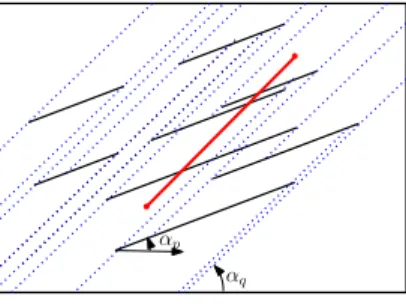
Third, we also provide an adjustable work-space algorithm for the segment intersection problems. Roughly speaking, the model of an adjustable work-space algorithm can perform with work-space of an arbitrary size betweenO(1) and O(n) words. Givennline segments in a plane, we invent adjustable work-space algorithms for detecting a segment intersection and for reporting all pairs of intersecting line segments. Specially, algorithm of detecting a segment intersection can be practical, which means that no complicated data structure is needed in the algorithm. We also obtain practical algorithms of reporting segment intersecting pairs for input ofcslopes line segments in which the input has at mostcdifferent slopes. In general, however,
the number of line slopes can ben. In this case, we have to use a sophisticated data structure.
Finally, we give polynomial-time algorithms for subgraph isomorphism problems for small graph classes of perfect graphs. This work comes from on the way that we try to design memory constrained algorithms for geometric graphs. So far, the memory constrained algorithms for the graphs have not be achieved yet. Although this work is out of the framework of memory constrained algorithms, we include into this paper as a future topics.
Key words: Computational geometry, Algorithms, Memory constrained algorithms, Space-Time tradeoffs
Contents
Abstract i
1 Introduction 2
1.1 Memory constrained algorithms . . . 2
1.2 Framework of memory constrained algorithms . . . 3
1.2.1 A constant work-space algorithm . . . 3
1.2.2 O(n) bits work-space algorithms . . . . 3
1.3 Adjustable work-space algorithms . . . 4
1.4 Paper organization . . . 4
2 Preliminaries 6 2.1 Computation model . . . 6
3 Constant work-space algorithm for farthest-point Voronoi Diagram 7 3.1 Notations and functions for farthest-point Voronoi diagram . . . 7
3.2 Functions for supporting constant work-space algorithm . . . 9
3.3 Applications of the algorithm . . . 10
3.4 How to cope with degeneracies . . . 12
3.4.1 Degeneracy caused by collinear points . . . 12
3.4.2 Degeneracy caused by cocircular points . . . 13
3.5 Concluding Remarks in Chapter 3 . . . 14
4 Depth-First Search UsingO(n)Bits 15 4.1 The DFS problem . . . 15
4.2 Related work . . . 16
4.3 Preliminaries . . . 16
4.4 Characterizations for the Gray and Black Vertices . . . 17
4.5 O(n) bits DFS Algorithms . . . 19
4.6 Tree-Walking . . . 21
4.7 DFS inO(logn)-Space for undirected Graphs withO(1)-Size Feedback Vertex Set . . . 22
5 Adjustable work-space algorithms for segment intersection problems 24 5.1 Segment Intersection Detection . . . 24
5.2 Segment Intersection Reporting . . . 25
5.2.1 Isothetic Segments . . . 26
5.2.2 Algorithm Using Property Partition . . . 27
5.2.3 Algorithm Using Filtering Search . . . 27
5.2.4 Segment Overlaps . . . 29
5.2.5 Segments of at MostcDifferent Slopes . . . 32
5.2.6 General Case . . . 32
5.3 Conclusions and Future Works of Chapter 4 . . . 34
6 Polynomial-Time Algorithms for SubgraphIsomorphismin Small Graph Classes of
Perfect Graphs 35
6.1 Introduction . . . 35
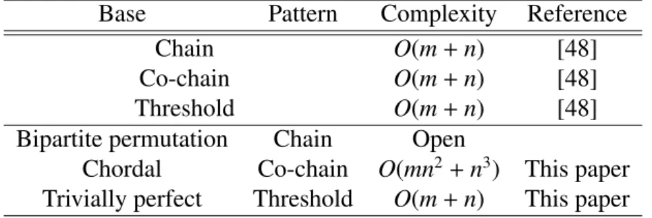
6.1.1 Our results . . . 36
6.1.2 Related results . . . 36
6.2 Preliminaries . . . 37
6.2.1 Definitions of the problems . . . 37
6.2.2 Graph classes . . . 38
6.3 Polynomial-Time Algorithms . . . 39
6.3.1 Finding co-chain subgraphs in chordal graphs . . . 39
6.3.2 Finding threshold subgraphs in trivially perfect graphs . . . 39
6.4 NP-completeness . . . 42
6.5 Conclusion of Chapter 6 . . . 44
Bibliography 45
Publications 50
Chapter 1 Introduction
There are increasing demands for highly functional consumer electronics such as printers, scan- ners, and digital cameras. To achieve this functionality they need sophisticated embedded soft- ware. One fundamental difference from software used in conventional computers is that there is little allowance of work-space which can be used by the software. Programs have been devel- oped under the assumption that sufficient memory space is available. The situation, however, asks us to design algorithms which work in small memory space.
1.1 Memory constrained algorithms
Work-space of an algorithm is a memory space used to store input data and results of temporary calculation for supporting its algorithm. To design memory constrained algorithms we assume that such work-space is given as a auxiliary space different from input and output space. Fur- thermore, we assume that input space is read-only space, and output space is write-only space, which means that those of space are not available as work-space.
Typically, the amount of work-space for an algorithm is limited into sublinear space for input data of length n, e.g. the work-space of size O(√
n) words. For example, there is a quite reasonable algorithm to use work-space of O(√
n) words for an binary image of size O(√
n) × O(√
n) [12]. Especially, one extreme sublinear constraints is to use only constant number of words. We just compute and maintain a constant number of words for input data consists ofnitems, and thus it takes work-space ofO(1) words of sizeO(logn) bits. Algorithms under this constraint have been extensively studied in complexity theory [5]. We call such algorithm aslog-space algorithmsorconstant work-space algorithmsin this paper.
We also consider more flexible usage of work-space for an algorithm than above constraint.
Work-space used in an algorithm for a problem involves its performance. Precisely, since there is tradeoffs between time and work-space for the algorithm, thus it runs in slower if less memory space is available. In theoretical sense, studies of time-space tradeoffs of an algorithm for a problem could give better comprehensions for its complexity rather than investigating only either time or space requirement. Many results for time-space tradeoffs have been appeared so far since early 1980s [59]. In particular, Beame and Borodin showed that lower bound for sorting problem of time-space product, which is the complexity of (running time of sorting)× (required space amount), under the machine model of branching program [17, 3]. Therefore, we also consider another memory constrained algorithms which can perform with a work-space of an arbitrary size. More precisely, work-space of the algorithm for input data of sizenis required in O(s) words, where s is parameter with 1 ≤ s ≤ n. We call such algorithms as adjustable work-space algorithms. In recent years, there are many adjustable work-space algorithms for geometric problems [52, 7, 41]. Chan and Chen provide algorithms for computing convex hull for givennpoints in a plane [22]. It is known as one of early adjustable work-space algorithms applied for geometric problems. Their algorithm outputs the convex vertices for input points in
the increasing order inO((n/s)(n+slogs)) time withO(s) words.
In this paper, we present memory constrained algorithms for geometric problems. We clas- sify the algorithms with type of the work-space following Section 1.2 and Section 1.2.2, respec- tively.
1.2 Framework of memory constrained algorithms
Instead of not using a large memory space, constant work-space algorithms could work on every machine. The algorithm can apply to process for massive data set such as so-called streaming algorithms [60]. On the other hand, however, the constraint to the constant work space seems too severe for practical applications. So, it is necessary to assume that much more work-space is available in algorithms rather than constant work-space.
1.2.1 A constant work-space algorithm
In this paper, we present limitted work-space algorithms for two fundamental problems. One of the them is that we present a constant work-space algorithm for drawing a farthest-point Voronoi diagram in Chapter 3. Farthest-point Voronoi diagram is obtained for a point set ofn points in a plane. The diagram partitions into unbounded regions surrounded by line segments and rays. Each region has a point pin the given set such that p is the farthest point from any point in its region.
It is usually described using a doubly-connected edge list, which can be computed inO(nlogn) time fornpoints. It supports the following operations
• To enumerate all Voronoi vertices,
• To enumerate all directed Voronoi edges,
• To determine whether a specified point is on the convex hull, and
• To follow the boundary of the Voronoi region for a point on the convex hull if we specify the point.
Once the doubly-connected edge list is constructed for a given set of pointsS of n points in O(nlogn) time usingO(n) work space, we can enumerate all vertices inO(1) time per vertex. In the constant work-space algorithm, with no preprocessing time we can enumerate all Voronoi vertices in O(n) time per each vertex. It is just the same for Voronoi edges. Following the boundary of a Voronoi region is also done inO(n) time per step.
1.2.2 O(n) bits work-space algorithms
The other constraint is somewhat relaxed from constant work-space algorithms. In Chapter 4, we investigate how one can perform Depth-First Search (DFS) of a given graph using limited amount of memory. DFS, being one of the most fundamental and important ways to search or explore a graph, is used as a subroutine in many prominent graph algorithms [70]. A better understanding of DFS in terms of space complexity and memory-efficient algorithms is desir- able, but it appears that such aspects of DFS have not been considered much. This is perhaps because the problem is trivial if one usesO(nlogn) bits of memory on one hand, wherenis the number of vertices of a graph, and, on the other hand, the problem isP-complete [65] and thus polylogarithmic-space algorithms are unlikely to exist.
1.3 Adjustable work-space algorithms
We propose adjustable work-space algorithms for segment intersection problems. The work- space is sublinear, however, work-space of the sizeO(s) words is available, wheresis parameter with 1≤ s≤n.
The problem has been well studied. Givennsegments in the plane, we can report allKinter- sections inO(nlogn+K) time if we can use work-space of sizeO(n) words. SinceΩ(nlogn+K) time is required in the worst case, the algorithm given by Balaban [15] achievingO(nlogn+K) time andO(n) words is optimal.
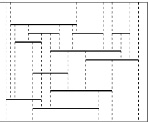
In Section 5.1 we begin with a simple adjustable work-space algorithm for segment inter- section detection, which runs in O((n2/s) logs) time using work-space ofO(s) words for a set of n line segments stored in a read-only array. Section 5.2 extends the result to the problem of reporting intersections usingO(s) work space. We present three different adjustable work- space algorithms all of which run in O((n2/s) logs+ K) time for a set ofn isotheticsegments (e.g. when given segments are horizontal or vertical). We need some special treatment if input segments may overlap each other, that is, if their intersection (in the mathematical sense) is a line segment, not a line. We show this problem can be resolved using techniques called filter- ing search given by Chazelle [25] . We also present an adjustable work space algorithm for a general set of segments with arbitrary slopes. The algorithm runs in roughlyO(n2/√
s+K) time.
We aim to design adjustable work-space algorithms so that it can be simple implementation into a program. Thus, algorithms should not be adopted complicated data structures such as multi-layer data structure [29]. Although our algorithm for segment intersection detection ap- plies for plane sweep algorithms provided by Bentley and Ottman [19], it is still quite simple.
We also aim to obtain deterministic algorithms. The product of time and space required in an algorithm for a problem should have an optimal lower bound. Considering memory constrained algorithms like adjustable work-space algorithm is helpful to understand for the study.
1.4 Paper organization
We present memory constrained algorithms for geometric problems in this paper. In Chapter 2, we define computation model on which our algorithms execute.
In Chapter 3, we propose memory constrained algorithms for fundamental geometric prob- lem, but it is not adjustable work-space. The problem is to find a farthest-point Voronoi diagram for givennpoints in a plane. In the chapter, we present constant work-space (i.e.O(logn) bits) algorithm for the problem. The algorithm consists of some functions which also perform using only constant work-space. Those functions are described in Section 3.2 with their implementa- tions. Especially, we can obtain an simple algorithm for an application of farthest-point Voronoi diagram, which is the problem of finding smallest enclosing circle. So, we give algorithms for drawing farthest-point Voronoi diagram and its application in Section 3.3.
We present another memory constrained algorithm in Chapter 4 for Depth-First Search, which traces all vertices and edges in depth-first order for a given graph withnvertices andm edges. We show that Depth-First search can implement using the work-space of sizeO(n) bits in Section 4.5. Furthermore, in Section 4.6 we provide also a constant work-space algorithm which performs Depth-First Search for spacial graphs of tree andO(1)-size feedback vertex set.
In Chapter 5, we present adjustable work-space algorithm for segment intersection prob- lems. Precisely, given n line segments in a plane, the objectives of the problem are to find
a segment intersection or to report all pairs of intersecting line segments. In Section 5.1 we present an adjustable work-space algorithm for the former problem which is called asSegment Intersection Detections, in Section 5.2 algorithms are given for the latter problem ofSegment Intersection Reporting, respectively. Both of the algorithms can work on the work-space of size O(s) words, where sis parameter with 1≤ s≤ n, which means an arbitrary size is available as its work-space.
In Chapter 6, as an additional work of this paper, we also give the results of the polynomial- time algorithms forSubgraph Isomorphismproblems. And we prove the NP-hardness of the Subgraph Isomorphism problem in small graph classes for perfect graph. It was supposed to consider designing memory constrained algorithms associated with some geometric graphs classes. It remains one of the future work.
Chapter 2
Preliminaries
2.1 Computation model
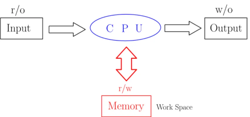
To design memory constrained algorithms, we define the computation model used in our algo- rithms (Fig 2.1). First of all, we assume that our algorithms run on the standard RAM model.
Thework-spaceis storages in which every stored element is allowed to be read, overwritten and removed. We measure the amount of work-space with the number ofwordsassociated with the size of input data. Work-space of a word is assumed to be large enough to store an input data or pointer. In this paper, we use the term of words for represent the amount of work-space.
Assuming that one word equals toO(logn) bits, we also use the term ofbitsto denote the size.
We also assume that the work-space is given different form input and output space.
In addition, we assume that input data of sizenis stored in a read-only array. So, no reorder- ing elements and overwriting in the array are possible while the algorithm is running. Output data is not stored in a memory space. Each element of output data is immediately reported when it is just generated. The facts imply the space of input and output storing are not available as the work-space. As a motivation of using read-only property, given input data, we may want to perform several different algorithms. If we reorder input points for an algorithm, then we have to reorder them for another one. For example, a good ordering for closet-point Voronoi diagram may be different from one for farthest-point Voronoi diagram. In fact, a problem of finding the minimum-width annulus for a set of points in the plane can be solved using both of the Voronoi diagrams. The topic is described in Section 3.3.
Input C P U Output
Memory
r/o w/o
Work Space
r/w
Figure 2.1: Diagram of computation model
Chapter 3
Constant work-space algorithm for farthest-point Voronoi Diagram
In this chapter, we presents a constant work-space algorithm for drawing a farthest-point Voronoi diagram. Voronoi diagram for a set ofnpoints in the plane, which is a collection of algorithms for supporting various operations on the diagram using only a constant number of words of O(logn) bits in addition to a read-only array to store the given point set. We show the oper- ations to be supported can be executed in O(n) time without using only constant work-space (without using any extra array). This is an extension of our previous results [6, 11, 14, 13].
3.1 Notations and functions for farthest-point Voronoi dia- gram
We define some notations for farthest-point Voronoi diagram and functions for supporting the constant work-space algorithm. We consider algorithm for a farthest-point Voronoi diagram FV(S) for a setS ofn points in the plane. For simplicity we assume that given points are in general positions, that is no four points ofS are cocircular and thus every vertex of FV(S) is incident to exactly three Voronoi edges. This restriction will be removed later. A diagram is defined by Voronoi regions and Voronoi edges. A Voronoi regionFVR(pi) for a point pi ∈S is the region such that the point pi is farthest among the point setS from any point in the region.
Each Voronoi region is known to be an infinite polygonal region, whose boundary consists of two infinite edges and (possibly no) finite edges with two endpoints. In this paper we orient Voronoi edges on the boundary of a Voronoi regionFVR(pi) so that the Voronoi region for the point pilies to their left. Each Voronoi edge lies between two Voronoi regions. So, byE(pi,pj) we denote a Voronoi edge between two Voronoi regionsFVR(pi) and FVR(pj) with FVR(pi) to its left (andFVR(pj) to its right). Thus, the oppositely directed edge, called the twin edge, is denoted by E(pj,pi). By our assumption exactly three Voronoi edges meet at each endpoint of Voronoi edges, which defines a Voronoi vertex. Thus, we can assume that each Voronoi vertex is characterized by three points from an input points such asV(pi,pj,pk).
It is well known that only those points of an input point set on its convex hull have their Voronoi regions [29, 64].
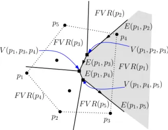
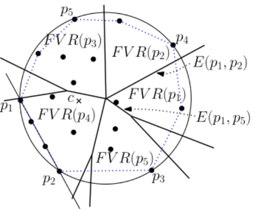
An example of a farthest-point Voronoi diagram is shown in Figure 3.1. In the figure, the leftmost point among the input points is denoted byp1and other input points on the convex hull are denoted by p2, . . . ,p5 in the counter-clockwise order. The Voronoi regionFVR(p1) for the point p1is shadowed in the figure.
A farthest-point Voronoi diagram is defined by Voronoi vertices, Voronoi edges which are either directed rays or directed line segments, and Voronoi regions which are infinite regions.
It is common to use a doubly-connected edge list (DCEL in short) to represent a farthest-point
p1
p2 p3
p4
p5
F V R(p1) F V R(p2)
F V R(p3)
F V R(p4)
F V R(p5)
E(p1, p2)
E(p1, p5) E(p1, p3)
E(p1, p4)
V(p1, p4, p5) V(p1, p3, p4) V(p1, p2, p3)
Figure 3.1: Farthest-point Voronoi diagram. Vertices on the convex hull are {p1, . . . ,p5}. FVR(pi) and E(pi,pj) are the Voronoi region for point pi and Voronoi edge for two points pi and pj, respectively.
Voronoi diagram. The DCEL consists of three collections of records [29].
Vertex record: A vertex record of a vertexvstores the coordinates ofvand a pointerIncidentEdge(v) to a directed edge outgoing ofv.
Face record: A face record of a face f stores a pointerFirstVoronoiEdge( f )to the first Voronoi edge on the boundary of the face f, which is a ray from the infinity.
Edge record: An edge record of a Voronoi edgeestores a pointerNextVoronoiEdge(e)to the next Voronoi edge on the same boundary and a pointerIncidentFace(e) to the face to its left.
We support these functions, IncidentEdge(v), FirstVoronoiEdge( f ), NextVoronoiEdge(e), andIncidentFace(e)by providing the following functions.
FirstExtremePoint(S) returns the leftmost extreme point (more exactly, the index of the point) in a setS of points.
CounterClockwiseNextExtremePoint(pi) returns the index of the extreme point next to piin a counter-clockwise order on the convex hull.
FrontEndpointOfVoronoiEdge(E(pi,pj)) returns the indexkof the point pk of S that deter- mines the front (terminating) endpointV(pi,pj,pk) of a directed Voronoi edgeE(pi,pj).
BackEndpointOfVoronoiEdge(E(pi,pj)) returns the index k of the point pk of S that deter- mines the back (starting) endpointV(pi,pj,pk) of a directed Voronoi edgeE(pi,pj).
NextVoronoiEdge(E(pi,pj),V(pi,pj,pk)) returns the next Voronoi edge E(pi,pk) of E(pi,pj) on the Voronoi region FVR(pi) which starts at the Voronoi vertex V(pi,pj,pk), more exactly the two indicesiandk.
ExtremePoint(pi) returns TRUE if and only if the point piis on the convex hull.
3.2 Functions for supporting constant work-space algorithm
We propose implementations of above functions for supporting our algorithm. Our constant work-space algorithm first computes the centroidcof the input point set in advance by comput- ing the averagexandycoordinates of all given points. It is well known that the centroid always lies in the interior of the convex hull for the point set.
The operations listed above can be implemented in linear time using only O(logn) bits as follows:
FirstExtremePoint(S): The leftmost point in a point set S must be on the convex hull of S since the left half plane defined by the vertical line through the leftmost point is empty (i.e., no point ofS is contained there). It is easy to find the leftmost point in S inO(n) time usingO(logn) bits.
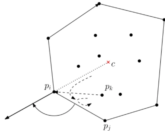
CounterClockwiseNextExtremePoint(pi): Let pi ∈S be an extreme point on the convex hull ofS. We define a ray emanating from the pointpiin the opposite direction to the centroid c (refer to Figure 3.2). Then, we rotate the ray in the counter-clockwise order until it encounters a point ofS, which is the point required. This is an intuitive description of an algorithm. Formally, we find the next extreme point pj as follows. The point pjmust satisfy the following two properties:
(1) (c,pi,pj) is clockwisely oriented since pj must be to the left of the directed line−−→cpi, and
(2) for any other point pk ∈S\{pi,pj}with the property (1) the three points pk,pi,pjare ordered clockwisely since pj lies to the left of−−−→pkpi to minimize the angle with the ray from pi(see Figure 3.2). Thus, it can be computed inO(n) time usingO(logn) bits.
FrontEndpointOfVoronoiEdge(E(pi,pj)): Each Voronoi edgeE(pi,pj) is associated with one or two enclosing circles, whose centers are the endpoints of the edge. Due to our orien- tation, the front endpoint of a Voronoi edgeE(pi,pj) is determined by a point ofS lying to the left of −−−→pipj. For each such point pk (such that (pi,pj,pk) is counter-clockwisely ordered) we compute the center of the circle through pi,pj, and pk. This is a kind of mapping of a point ofS into one on the perpendicular bisector of pi and pj. The center point giving the front endpoint must give an enclosing circle as stated above. Thus, the center point must be farthest from the center point of piandpj. Thus, it can be computed inO(n) time usingO(logn) bits. See Figure 3.3. It shows how to find such a point. Given a Voronoi edge E(p1,p3), extreme points of S lying to the left of the directed line−−−→p1p3 are p4 and p5. Since p4 corresponds to a larger circle, the front endpoint of the edge is determined by p4together with p1andp3in this example. It should be noted that the last Voronoi edge on the boundary of a Voronoi region when we traverse it counterclockwisely has its front endpoint at infinity and thus its front endpoint is undefined.
BackEndpointOfVoronoiEdge(E(pi,pj)): This is just symmetric to the case of the front end- point. Thus, the first Voronoi edge on the boundary of a Voronoi region has no back endpoint.
NextVoronoiEdge(E(pi,pj),V(pi,pj,pk)): Once Voronoi edgeE(pi,pj) and its front endpoint V(pi,pj,pk) are known (more exactly, three indicesi, j,andkare known), the next Voronoi edge isE(pi,pk). Thus, it is done inO(1) time.
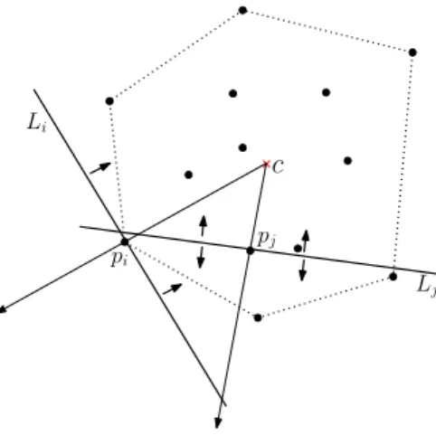
ExtremePoint(pi) We can easily compute the line Li that is perpendicular to the ray from the centroid c toward pi. If one of the half plane contains no point of S except pi on the boundary, then the point pi is on the convex hull by the definition of the convex hull.
Otherwise, it is an interior point. See Figure 3.4. This is done inO(n) time.
In addition, given a Voronoi edge E(pi,pj) and its front endpoint V(pi,pj,pk), we know the three Voronoi edges E(pj,pi),E(pi,pk) andE(pk,pj) are outgoing edges from the Voronoi vertex V(pi,pj,pk) ordered in a clockwise way around the vertex. Thus, the algorithm above behaves like a doubly-connected edge list.
pi
c
pj
pk
Figure 3.2: Finding the counter-clockwise next extreme point using a ray from pi and the cen- troidc.
p1
p2 p3
p4
p5
F V R(p1) F V R(p2)
F V R(p3)
E(p1, p3)
V(p1, p3, p4) V(p1, p2, p3)
Figure 3.3: Finding the front endpoint of a Voronoi edge which is determined by a point of S lying to the left of the directed linep1p3. Points lying to the directed linep1p3arep4andp5. The center point of the circle defined by (p1,p3,p4) is farther than that defined by (p1,p3,p5), and thus the front endpoint of the directed Voronoi edgeE(p1,p3) is the Voronoi vertexV(p1,p3,p4).
On the other hand, only one point p2lies to the directed line p3p1, and thus that ofE(p3,p1) is V(p3,p1,p2)= V(p1,p2,p3).
3.3 Applications of the algorithm
Using the constant work-space algorithm for farthest-Point Voronoi diagram, we can of course draw the diagram for any given set ofn points inO(n2) time using only O(logn) bits given as
pi
c
pj
Li
Lj
Figure 3.4: Deciding whether a given point is on the convex hull. The point pi is on the convex hull shown by dotted lines since one of the half plane defined by the lineLiis empty. The point pj is not so since none of the half planes is empty.
Algorithm 1 below.
A constant-work-space algorithm for drawing the farthest-point Voronoi diagram
Input:A setS ={p1, . . . ,pn}ofnpoints.
Output:Voronoi edges and Voronoi vertices of the farthest-point Voronoi diagram of the setS. Algorithm{
pi=FirstExtremePoint(S).
i0 = i. repeat{
pj =CounterClockwiseNextExtremePoint(pi).
pk =FrontEndpointOfVoronoiEdge(pi,pj).
Report the first Voronoi edgeE(pi,pj) ema- nating from the Voronoi vertexV(pi,pj,pk).
repeat{ pj = pk.
pk=FrontEndpointOfVoronoiEdge(pi,pj).
if(pkis undefined)thenexit the loop.
Report the Voronoi edge (segment) E(pi,pj) (pair of indicesiand jin practice) and the Voronoi vertexV(pi,pj,pk) together with its coordinates and three indices.
}(forever) }until(i=i0)
Report the last Voronoi edge (ray) E(pi,pj) emanating from the last Voronoi vertex.
pi=CounterClockwiseNextExtremePoint(pi).
}
We can also compute the smallest enclosing circle of the points set by enumerating all the Voronoi vertices and Voronoi edges in O(n2) time. The smallest enclosing circle for a
point setS is defined either by three points associated with a Voronoi vertex or by a diametral pair of extreme points. In the former case the point must appear as a Voronoi diagram of the farthest-point Voronoi diagram. In the latter case, the diametral pair of points mus appear as one associated with a Voronoi edge. Thus, if we enumerate all Voronoi vertices and Voronoi edges, we can find the center of the smallest enclosing circle. Since there areO(n) Voronoi vertices and edges, the algorithm runs inO(n2) time.
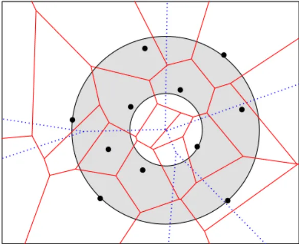
Another application is to the smallest annulus of a point set. Given a setS ofnpoints in the plane, two co-centric circles are called an annulus ofS if all the points ofS lie between the two circles. See Figure 3.5. The width of an annulus is the difference of the two radii.
There are two cases to determine the center of the smallest-width annulus. In one case one of the circles is determined by three points and the other by a single point. In the other case both of them are determined by two points. The center in the latter case is given as an intersection of two Voronoi edges, one from the closest-point Voronoi diagram and the other from the farthest-point Voronoi diagram ofS [33]. An algorithm for enumerating all the edges of the closest-point Voronoi diagram inO(n2) time usingO(logn) bits is available [13]. Thus, a straightforward algorithm is to enumerate all edges of the farthest-point Voronoi diagram for each edge in the closest-point Voronoi diagram and to check intersection of those edges from different Voronoi diagrams. This algorithm runs inO(n4) time andO(logn) bits.
Figure 3.5: The minimum-width annulus for a set of points. The closest-point and farthest point Voronoi diagrams are drawn in solid and dotted lines, respectively, in the figure.
3.4 How to cope with degeneracies
We have assumed that given points are in general positions, that is, (1) no three points are on a line or (2) no four points are on a circle. In this section we will show how to cope with degeneracies on given points.
3.4.1 Degeneracy caused by collinear points
Figure 3.6 shows an example of a degeneracy caused by collinear points in which four points lie on the convex hull of a given point set.
Suppose three points from an input point setS lie on a line and one of the half plane defined by the line is empty, that is, it contains no point ofS. If three pointspa,pb, and pcare arranged in this order on the line, the middle point pb never contributes to the farthest-point Voronoi
c
pi
pj
pk
pj
Figure 3.6: Degeneracy caused by collinear points.
diagram for S, in other words, pb has no its own Voronoi region, for any circle touching pb never includes both of pa and pc, and the point pa(resp., pc) lying outside the circle is farther from the center of the circle than the other point pc (resp., pa). This means that we can neglect those intermediate points on the convex hull edges, which are not convex hull vertices. All these observations lead to the following algorithm forCounterClockwiseNextExtremePoint(pi):
CounterClockwiseNextExtremePoint(pi) foreach point pk ∈S\{pi}do
if(c,pi,pk) is counter-clockwisethen break;
foreach point pj, j= k+1, . . . ,ndo if(c,pi,pj) is counter-clockwisethen
if(pk,pi,pj) is counter-clockwise then pk = pj;
else if(pk,pi,pj) is collinearand(c,pk,pj) is counter-clockwisethen pk = pj;
return pk.
3.4.2 Degeneracy caused by cocircular points
Figure 3.7 shows another type of degeneracy, which is caused by cocircular points. In the figure five points p1, . . . ,p5on the convex hull lie on a circle.
p1 c
p2 p3
p4 p5
F V R(p1) F V R(p2) F V R(p3)
F V R(p4)
F V R(p5)
E(p1, p2)
E(p1, p5)
Figure 3.7: Degeneracy caused by cocircular points.
Suppose we are about to examine a convex hull edge (p1,p2). We first find a Voronoi edge E(p1,p2), which is a ray from the infinity, as shown in the figure. To compute its front endpoint
we examine all the points lying to the left of the directed line from p1 to p2 to find one whose corresponding circle center is farthest from the middle point of p1andp2. In this case the three points p3,p4 andp5 all give the same circle center since they are cocircular. Note that all those points must be extreme points. What we want is the point closest to p2 in the clockwise order on the convex hull. Thus, if we find two candidate extreme points paand pb to define the front endpoint of a Voronoi edge E(pi,pj) and the four points pa,pb,pi and pj are cocircular, then we check the orientation of (pi,pa,pb). We choose pa if it is counter-clockwise, and choose pb otherwise. This extra condition leads to a correct ordering of those cocircular points. In the example of Figure 3.7, the front endpoint ofE(p1,p2) is defined byp3, and thus the next Voronoi edge should beE(p1,p3). Its front endpoint is defined byp4and thus the following edge should be E(p1,p4). In the same manner the Voronoi edge E(p1,p4) is followed by E(p1,p5). So, we have an edge sequenceE(p1,p2),E(p1,p3),E(p1,p4),E(p1,p5). Here note that the Voronoi edgesE(p1,p3) andE(p1,p4) are degenerated edges, that is, their two endpoints coincide.
3.5 Concluding Remarks in Chapter 3
We have presented a constant work-space algorithm for a farthest-point Voronoi diagram, which is a collection of algorithms to execute all of operations associated with the diagram as effi- ciently as possible using only constant work-space. A number of problems are left open. One of them is to establish some trade-offbetween running time and amount of work-space. Given work-space ofO(s) words, how fast can we compute a farthest-point Voronoi diagram? It is not known whether we can establish time complexity such asO(n2/s) orO(n2/slogn). To answer this question we need to devise a algorithm usingO(s) space withs∈o(n). One typical question is how fast can we draw a farthest-point Voronoi diagram for a set ofnpoint in the plane using the work-space of sizeO(√
n) words.
Chapter 4
Depth-First Search Using O(n) Bits
We provide algorithms performing Depth-First Search (DFS) on a directed or undirected graph with n vertices and m edges using only O(n) bits. One algorithm usesO(n) bits and runs in O(mlogn) time. Another algorithm usesn+o(n) bits and runs in polynomial time. Furthermore, we show that DFS on a directed acyclic graph can be done in work-spacen/2Ω(
√logn)bits and in polynomial time, and we also give a simple linear-timeO(logn) bits algorithm for the depth- first traversal of an undirected tree. Finally, we also show that for a graph having anO(1)-size feedback set, DFS can be done inO(logn) bits work-space. Our algorithms are based on the analysis of properties of DFS and applications of thes-tconnectivity algorithms due to Reingold and Barnes et al., both of which run in sublinear space.
4.1 The DFS problem
Before we outline previous work on DFS, we explain some technical details about the DFS problem. We can cast a DFS problem in various ways. The output can be (1) the DFS tree, or the output can be (2) the DFS numbering of each vertex, that is, the ordering of vertices with respect to the time of the first visit, or (3) the input can be a graph together with two verticesu andv, and the output can be the yes/no answer as to whether vertexuis visited before vertexv in DFS. For our purposes, which of the three variants above we consider does not matter since they can all be reduced to each other using O(logn) bits. Furthermore, all the algorithms we present can directly handle any of the three variants in a straightforward way. For definiteness, we think of DFS problem as the DFS tree construction problem.
We assume that an input graph is given by an adjacency list. Suppose that DFS is visiting a vertex v for the first time, reaching v from vertex u. DFS will now visit the first unvisited neighbor ofv, where the “first” is usually with respect to either one of the following two orders:
(1) the appearance order in v’s adjacency list; or, (2) in the case of undirected graphs: under the assumption that n vertices are numbered 1, . . . ,n and with respect to the cyclic ordering of 1, . . . ,n, the unvisited vertex x amongv’s neighbors that appears first after u in the cyclic ordering.
DFS with respect to either one of the two scenarios above is sometimes calledlexicograph- ically smallest DFSorlexicographicDFS orlex-DFS[30], [31] (and sometimes simply called DFS). Usually, a lex-DFS algorithm can handle both scenarios (1) and (2) in the same manner, and one does not need to distinguish the two scenarios. All algorithms in this paper perform lex-DFS.
In contrast to lex-DFS, we can also consider an algorithm that outputssomeDFS tree of a given graph. Such an algorithm treats an adjacency list as aset, ignoring the order of appearance of vertices in it, and outputs a spanning tree T such that there exists someadjacency ordering R such thatT is the DFS tree with respect toR. We say that such a DFS algorithm performs general-DFS.
4.2 Related work
This paper is concerned with the more classical Random Access Machine (RAM) model, where input data is in read-only random access memory, and computation proceeds using additional working space, which, for example, consists of O(logn) or o(n) or O(n) bits. The output will be stored in a write-only output tape. For this model, recent works have given some new inter- esting memory-limited algorithms: Elberfeld et al. [34] and Elberfeld and Kawarabayashi [35]
have givenO(logn) bits algorithms for solving a family of fundamental graph problems (more precisely those problems expressibly in monadic second-order language on graphs of bounded tree-width) and for the canonization of graphs of bounded genus. Very recently, Asano et al. [10]
and Imai et al. [47] have shown that the reachability problem on directed graphs can be solved using only ˜O(√
n) words for planar graphs.
Reif [65] has shown that lex-DFS is P-complete. Anderson and Mayr [4] have shown that computing the lexicographically first maximal path, that is, computing the leftmost root-to-leaf path of the lex-DFS tree, is already P-complete.
Aggarwal and Anderson [2] have shown that general-DFS is computable in RNC, that is, computable by a randomized parallel algorithm with polynomially many processors and in poly- logarithmic parallel time in the PRAM model, or, equivalently, by randomized polynomial-size poly-logarithmic depth circuits. There is no known deterministic NC algorithm for general- DFS.
In a seminal work, Reingold [66] has given a deterministicO(logn) bits work-space algo- rithm for the Undirecteds-tConnectivity Problem:
Theorem 1 (Reingold [66]) Given an undirected graph and two vertices s and t, determining whether s and t are connected can be done in deterministic O(logn)bits.
Using Reingold’s algorithm, one can compute a minimum spanning tree of a given graph in O(logn) bits.
The s-t connectivity problem for directed graphs is NL-complete. This problem can be solved using O(log2n) bits and nO(logn) time by Savitch’s algorithm (see [62]). Concerning polynomial-time algorithms solving this problem, the best known upper bound for space is the following slightly sublinear one due to Barnes et al. [16]:
Theorem 2 (Barnes et al. [16]) Directed s-t connectivity can be solved deterministically in work-space n/2Ω(
√logn)bits and in polynomial time.
This is also the best space upper bound for polynomial-time algorithms solving the following problems: computing the distance between a vertexsand a vertextin an undirected or directed unweighted graph, computing the single-source shortest-path tree in a weighted undirected or directed graph [46], and a computing the breadth-first search tree.
4.3 Preliminaries
Throughout the paper, we assume that the set of vertices of a given graph is the set{1, . . . ,n}. We think of DFS in the following way: Initially, all the vertices are white. When vertexv is visited from vertexu, the color ofvchanges from white tograyand thesearch headmoves from u tov. When there is no more white neighbor ofv, the search atvis finished, the color of vchanges from gray toblack, and the search headreturns fromvto u.
Suppose that in a given undirected or directed graph,mvertices are reachable from the DFS starting vertex s. At time t = 0, all vertices are white. At time t = 1, the starting vertex s becomes gray. At each timet ≥ 1, exactly one vertex changes its color, either from white to gray, or, from gray to black. At time t = 2m, the color of s becomes black and the search is completed. For a vertex v, the discovery time of v is the time when v changes its color from white to gray and thefinishing timeis the time whenvchanges its color from gray to black.
Note that the gray vertices always form a simple path from the starting vertexsto the vertex where the search head is currently located. We can also think of this path as residing in the depth-first-search tree.
We let Reachable(x,u,G) denote a subroutine that decides, given a graphGand two vertices xandu, whether vertexuis reachable from vertexxinG. IfGis a directed graph, reachability is interpreted in terms of a directed path, and ifGis undirected, it simply means connectivity.
To implement Reachable(x,u,G) we apply Reingold’s algorithm and Barnes et al.’s algorithm for the cases of undirected and directed graphs, respectively.
4.4 Characterizations for the Gray and Black Vertices
In this section, for the sake of convenience, we collect our lemmas characterizing the gray vertices, the gray path, and the black vertices in several settings. These lemmas naturally yield our algorithms in the next section and they are crucial to explain their correctness. For most lemmas, proofs are immediate and omitted.
Lemma 3 (All-White Path) Vertex v is visited during DFS while vertex u is gray, (i.e.,v is a descendant of u in the DFS tree) if and only if the following holds: At the time u is discovered, vis white andvcan be reached from u by an all-white path.
Let sbe the starting vertex of a DFS. In the following we assume that the state of the DFS at timetis such that the search head is at a gray vertexu. Let p=⟨i0 = s,i1, . . . ,ik−1,ik =u⟩be the gray path at timet, whereij+1is visited fromij (for 0≤ j< k).
The following lemma characterizes the gray path in terms of black vertices.
Lemma 4 (Gray Path from Black Vertices) The gray path p = ⟨i0 = s,i1, . . . ,ik−1,ik = u⟩ satisfies the following. For j∈ {0, . . . ,k−1}, vertex ij+1is the first vertex x in the adjacency list of vertex ij such that (1) x is not black at time t, and that (2) x is not in{i0, . . . ,ij}.
Proof. Vertexij+1becomes gray only after all the vertices in the adjacency list ofij preceding
ij+1have become non-white. 2
LetC = {i0, . . . ,ik}be the set of gray vertices comprising the gray path P. The following characterization explains how to reconstruct thepath Pfrom theset C.
Lemma 5 (Gray Path from Gray Set) Let P′ = ⟨i0, . . . ,ij⟩ be the initial segment of P of length j. Then, the following characterizes the immediate successor x=ij+1of ij in P.
(1) x is in C.
(2) x is a neighbor of ij. (3) x is not in{i0, . . . ,ij}.
(4) x is the first vertex in the adjacency list of ij satisfying (1), (2), and (3).
For our algorithms we need to be able to reconstruct the gray pathp=⟨i0 = s,i1, . . . ,ik−1,ik = u⟩ from the two endpoints s and u alone. The following lemma characterizes the vertices i1, . . . ,ik−1 in such a way that one can reconstruct them given sandu. The proof immediately follows from Lemma 3 (All-White Path).
Lemma 6 (Gray Path) For j ∈ {1, . . . ,k− 1}, vertex ij is the first vertex x in the adjacency list of ij−1 from which vertex u can be reached without going through any of the vertices in {i0, . . . ,ij−1}.
Corollary 7 (Gray Path Reconstruction) Using an n-bit vector one can reconstruct i1, . . . ,ik−1 one by one as follows. For j=1, . . . ,k−1, for each vertex x adjacent to ij−1, use Reachable(x,u,G− {i0, . . . ,ij−1})and the previous lemma to determine whether x is ij.
When considering DFS on a DAG the characterization and reconstruction of the gray path simplifies as follows.
Lemma 8 (Gray Path in a DAG) For j ∈ {1, . . . ,k −1}, vertex ij is the first vertex x in the adjacency list of ij−1such that vertex u is reachable from x.
Proof. LetPbe a directed simple path fromxtou. Then no vertexyin{i0, . . . ,ij−1}can appear on the pathPsincexis reachable fromyand the graph is acyclic. 2 Corollary 9 (Gray Path Reconstruction in a DAG) For a DAG, one can reconstruct i1, . . . ,ik−1 similarly as in the Gray Path Reconstruction Corollary above but without keeping track of i0, . . . ,ij−1by replacing the call to the routine Reachable(x,u,G−{i0, . . . ,ij−1})with Reachable(x,u,G).
Let sbe a starting vertex of a DFS. Assume that at timet−1, the gray path is of the form
⟨i0 = s, . . . ,ik = u,ik+1 = v⟩, and that at timet, vertex v gets finished, and thus the gray path is now of the form⟨i0 = s, . . . ,ik = u⟩. Let the adjacency list of vertexu be⟨l1, . . . ,lq−1,lq = v,lq+1, . . . ,lr⟩. DFS has backtracked from v to u and now we want to find the first unvisited, white vertex xamonglq+1, . . . ,lr in order to visit xnext. If we find out that such an xdoes not exist, we backtrack further fromu.
Suppose y ∈ {lq+1, . . . ,lr}. We can determine whether y has been visited or not, that is, whetheryis black, gray or white using the following lemma.
Lemma 10 (Black Vertex in a Directed Graph) Vertexyis black at time t if and only if there exist j∈ {0, . . . ,k}and vertexαsuch that the following hold:
1. The directed edge(ij, α)exists.
2. In the adjacency list of ij, vertexαprecedes vertex ij+1.
3. Vertexyis reachable from vertexαwithout going through any of the vertices{i0, . . . ,ij}. Proof. Vertexyis black if and only if the path from stoyin the DFS tree is lexicographically smaller than the path fromstou. We can easily finish the proof using the Lemma 3 (All-White
Path). 2
For undirected graphs, we can simplify the lemma above as follows.
Lemma 11 (White-Black Not Adjacent in Undirected DFS) During a DFS in an undirected graph, a white vertex is never adjacent to a black vertex.
Proof. Initially, the property holds, and the property is maintained during DFS since a vertex becomes black only when all of its neighbors are non-white. 2 Lemma 12 (Black Vertex in an Undirected Graph) Vertex yis black at time t if and only if the following holds: There exists a vertex w ∈ {l1, . . . ,lq−1} such that y is reachable from w without going through{i0, . . . ,ik}.
Proof. When vertex u is first visited from ik−1, none neighbor of us is black by Lemma 11 (White-Black Not Adjacent in Undirected DFS), and hence jandα, as required in Lemma 10 (Black Vertex in Directed Graph), cannot exist if j< k. 2
4.5 O(n) bits DFS Algorithms
Our algorithms maintain the color of each vertex. For example, our 4-color algorithm uses 2 bits per vertex to hold the current color and thus uses 2n bits in total for color information.
Any additional space used iso(n) bits, and thus the space used to maintain the colors dominates the space complexity of our algorithms.
A basic problem that we face when restricted toO(n) bits work-space is that we cannot store, for example, the ordered list of the vertices that are currently gray since that would require work- space of sizeΘ(nlogn) bits. A basic solution is to retrieve information by restarting the search from the starting vertex.
Algorithm 1: a 4-Color Algorithm. Our first algorithm, Algorithm 1, uses 4 colors for each vertex. It uses white, gray, and black according to the definitions of these colors explained in Section 2. To backtrack, it retraces the current gray path using Lemma 5 (Gray Path from Gray Set) by using one new color, blue, to keep track of the gray vertices in the initial segment reconstructed so far. We describe the algorithm in greater detail. Initially the starting vertex is colored gray and all other vertices are colored white. Suppose during the DFS we are at a vertexu(which must then be gray). Ifuhas a white neighbor then we proceed with the search going to the first white neighbor ofu, which is then colored gray. Ifuhas no white neighbor, we colorublack and backtrack. When backtracking, in caseuis the starting vertex the search ends. Otherwise we need to determine the parent ofuwhich is done by retracing the gray path as follows. We color the starting vertex blue. Then we repeatedly find the smallest gray vertexv that is a neighbor of the last vertex that was colored blue until this vertex isu. Whenuis colored blue, the parent of uis the last vertex that was colored blue just before that. We then recolor all blue vertices to be gray (by once again retracing the path), recoloruto be black, and have successfully backtracked.
Theorem 13 Given an undirected or directed graph G consisting of n vertices and m edges, DFS on G can be done in O(mn)time and in work-space2n+O(logn)bits.
Proof. As explained in Section 4.3, the total number of color changes is 2n. Between any two
color changes, each edge is inspected at mostO(1) times. 2