JAIST Repository: Measuring Financial Crisis Index for Risk Warning through Analysis of Social Network

(1)

Japan Advanced Institute of Science and Technology

JAIST Repository

https://dspace.jaist.ac.jp/

Title Measuring Financial Crisis Index for Risk Warning through Analysis of Social Network

Author(s) 王, 忠聖

Citation

Issue Date 2018-03

Type Thesis or Dissertation Text version author

URL http://hdl.handle.net/10119/15170 Rights

Description Supervisor:白井清昭, 先端科学技術研究科, 修士

(2)

Measuring Financial Crisis Index for Risk Warning

through Analysis of Social Network

WANG ZHONGSHENG

School of Advanced Science and Technology

Japan Advanced Institute of Science and Technology

(3)

Master’s Thesis

Measuring Financial Crisis Index for Risk Warning

through Analysis of Social Network

1610025 WANG ZHONGSHENG

Supervisor Kiyoaki Shirai

Chief Examiner Kiyoaki Shirai

Examiner Hiroyuki Iida

Nguyen Minh Le

Shogo Okada

School of Advanced Science and Technology (Information Science)

Japan Advanced Institute of Science and Technology

(4)

Abstract

With the growth of globalization, the association among countries of trading and financial markets are more intimate than before. However, since a stock market is quite, innate complex, dynamic, and chaotic, management of financial risk has been proved to be a very difficult task. For many decades, many researchers tried to analyze historical stock prices or financial statements of companies to measure financial risk. But the results were still not quite helpful for risk management.

The goal of this research is to propose a new financial index that measures an extent of a financial crisis. Microblog is used as a source of our new index. Hypotheses behind our financial crisis index are as follows. In Socioeconomic Theory of Finance, irrational speculation behaviors play an important role in a financial risk. First, not many investors pay attention to financial markets daily. When a bull market begins and stock price keeps going up, more beginners come into markets. Second, those people are intense to take irrational speculation behaviors. It may cause a panic and a bear market. Behaviors of beginners may make a financial risk more serious. Third, when many novice investors come into the market, they posts messages about financial topics. Therefore, intensity of attention toward finance on microblog may has a positive correlation with a financial bubble level. Fourth, this index can be used as an observable financial market singularity for a risk management.

Following these hypotheses, this thesis proposes Financial Attention Index, which is a new index for measuring financial crisis. It is defined as proportion of the financial related comments to the total number of comments on microblog. As discussed before, we suppose that financial topics are to be more mentioned and discussed on microblog when many novice investors participate in the market. Such a situation might cause the market unstable. Therefore, FAI is supposed to be positively correlated to a financial risk. Comments on microblog are classified whether they are related to financial topics or not. Weibo is chosen as SNS in this study. Then the number of financial comments and total comments are counted to get FAI. A classifier of financial related comments is not trained from Weibo comments, since it is difficult to prepare a large amount of labeled Weibo comments for supervised machine learning. Instead, a labeled data of news articles is used for training.

In this thesis, two kinds of financial classifiers are trained. One is the “Two-way classifier”, it classifies a comment on Weibo as a financial or non-financial related comment. The other one is “Three-way” classifier, it classifies a comment on Weibo into three classes: The first one is “stock-related”, which is a comment just related to the stock market. The second one is “financial-related”, which is a comment related to financial markets such as future market, bond market and so on, but not related to the stock market. The third one is “other”, which is a comment not related to financial topics. Since we mainly focus on analysis of stock prices for detection of a financial crisis, we distinguish topics about stocks with other financial related topics. When the three-way classifier is used for calculation of FAI, both stock-related and financial-related comments are treated as the financial comments.

Support Vector Machine to classify the comment on microblog in this study. Bag-of-words are used as features for training SVM. Function words are removed by a preprocessing and all content words in a document are extracted as the features. The weight of each feature is set as the TF-IDF score. We found that the number of the features was high. Therefore, we applied Latent Semantic Analysis (LSA) to reduce the feature space.

In addition, we try to use our proposed financial crisis index to predict a financial market trend for a risk management. FAI is used for prediction of a stock index to evaluate its ability for risk management. SSE Composite Index (SCI) is chosen as the index to be predicted, because our FAI is derived from comments of Weibo that is Chinese microblogging service and SCI is computed from prices of stocks of Chinese companies. LSTM is chosen for training a

(5)

prediction model, since it is well used for prediction of time series. In our model, input of LSTM is a time sequence of either the stock index, a difference of the stock index, or FAI. The difference of the stock index is defined as a change of the stock index between the current and previous periods. The output of LSTM is a stock index of the next period. We define a period of LSTM as one transaction day. Note that FAI is calculated for each week. If FAI is used for LSTM, the same value is entered during days in a week. We also train two models where three kinds of inputs are used simultaneously as the input. First is a simple model, where three values are concatenated as a vector and passed to the input layer of LSTM. Second is a multi-layer LSTM with multiple inputs, where three values are inputed sequentially in stacked LSTMs.

Several experiments are conducted to evaluate our proposed methods. First, the classifier to distinguish financial-related and other comments on Weibo is evaluated. Next, LSTM-based stock price prediction model is evaluated. In this experiment, our model is evaluated for its ability to predict not the stock index but a movement of the stock index (“Up”, “Down” or “Keep”). Two evaluation criteria are used in this experiment. The first evaluation criteria is “Accuracy”, which is a proportion of the number of the test periods for which the predicted movement class agrees with the true class. The second one is “No Lost Accuracy”. The main goal of this research is to help investors not to get a good return but to avoid financial risks. It is more important to predict the movement “Down” in order not to cause loss. Therefore, No Lost Accuracy is introduced, which is the accuracy of the stock movement prediction task where the test periods are classified as either “Down” or not. That is, “Up” and “Keep” classes are merged into one class “Not-Down”.

In overall prediction results, the difference of the stock index (DI) has the best performance both in “Accuracy” and “Not Lost” two evaluation criteria. The different situation prediction results of the experiment show a tendency that the model “FAI” achieves better performance than the others in the situations of both a bull and bear market. Especially, it is good on a front bull situation. These results indicate that FAI is effective to predict a drastic movement of the market. On the other hand, the model using the difference of the stock index (DI) works well for the stable situations. The model using the stock index (SI) is the worst in our experiment. Finally, it is found that multi-layer LSTM with multiple inputs performed very poorly.

Although a financial crisis can be measured by various points of view, this thesis showed that FAI could be a financial crisis index from one perspective. In future, since the result of the multi-layer LSTM with multiple inputs were not good, we will investigate a better design of a structure of LSTM to accept multiple inputs, i.e. the stock index, the difference of the index, and FAI.

(6)

Acknowledgment

I am greatly thankful to my supervisor, Associate Professor Kiyoaki Shirai for his gentle en-couragement and instruction for my Master course. He has always inspired me in my research. I could not finish this work and get any achievement without his support. It was a pleasure to work with him.

I also would like to thank Professor Hiroyuki Iida, Associate Professor Nguyen Minh Le of JAIST for their valuable comments and advises during the time I have been studying and doing my research in JAIST. Professor Hiroyuki Iida and Associate Professor Nguyen Minh Le have kindly gave my research good advice and some inspiring questions. It was quite helpful in my research and receive expensive knowledge from a different perspective.

A special thank to my friends who always believe in me, make me confident in myself and being with me during hard time. Panuwat Assawinjaipetch, OU WEI and LIANG YUBIN have brought me a lot of useful advises in daily activities and aided me to understand topics in my courses. WANG ZHENYU and Kento Kobayashi have helped me to improve my communication skills and gave me significant comments and advises for my presentations, writing and research. I also want to thank HUANG JINFENG, LIN WENSHENG and HU GUOXIN due to their presence, encouragement and sharing throughout my difficult life in a foreign country. I also want to say a sincere thank to SHEN TAO who provided me with valuable guidance and helpful advises to move on when I faced to a stressful unexpected situation without having the presence of my parents in Japan. All of them make me feel like a member of family and have another home in JAIST. It is not easy to find such great friends when living outside of my country, China, and having their support throughout a long duration. I am very grateful to be their friend.

Finally, I want to say the deepest thanks to my family for the unconditional love and contin-uous support. Based on the constant encouragement from my family and especially important guidance from my mother, I can follow my dream of doing research and chase goals of my life. It was because of my family, I could continue my study under pressure of research and stress of the unexpected situation and finally got an academic degree in Japan. I am very thankful for their presence. I would like to consecrate my work to my family for their endless love, support and encouragement throughout my life.

(7)

List of Figures

1.1 Hypothesis of financial attention . . . 3

2.1 Methodology of stock price prediction with LSTM[21] . . . 5

2.2 Graphical model representation of TSLDA [23] . . . 6

2.3 Methodology of sentiment-aware stock prediction [16] . . . 7

3.1 Procedure to calculate FAI . . . 9

3.2 Support Vector Machine for classification . . . 13

3.3 Support Vector Machine definition . . . 13

4.1 Overview of Long Short Term Memory [33] . . . 14

4.2 Overview of LSTM with multiple inputs . . . 16

4.3 Multi-input and multi-output model of LSTM [4] . . . 17

4.4 Multi-layer LSTM with multiple inputs . . . 18

5.1 Common use of test and training data . . . 21

5.2 Use of test and training data in this experiment . . . 22

5.3 Change of loss function in terms of epoch . . . 22

5.4 Result of multi-layer LSTM in the first term . . . 23

5.5 Result of multi-layer LSTM in the eighth term . . . 24

5.6 Fluctuation of SCI in dataset . . . 25

5.7 Twelve terms of different situations . . . 25

5.8 Stable range . . . 26

5.9 Bull range . . . 26

5.10 Bear range . . . 27

5.11 stock period table . . . 27

5.12 Comparison between SCI predicted by model SI and true SCI (second period) . 28 5.13 Comparison between SCI predicted by model SI and true SCI (235th period) . . 33

A.1 Algorithm to obtain word list . . . 40

A.2 Source code to obtain word list . . . 41

A.3 Algorithm to create dictionary . . . 41

A.4 Source code to create dictionary . . . 42

A.5 Algorithm to calculate TF-IDF . . . 43

A.6 Source code to calculate TF-IDF . . . 44

A.7 Algorithm of LSA . . . 45

A.8 Source code of LSA . . . 45

A.9 Python libraries to train LSTM . . . 46

A.10 Layer merging of Multi-layer Input LSTM . . . 47

(10)

List of Tables

3.1 News dataset . . . 11

5.1 Result of classification of financial comments . . . 19

5.2 Result of F -test . . . 20

5.3 Results of the stock movement prediction . . . 24

5.4 Prediction for different situations . . . 28

5.5 MSE between real and predicted index (1st-40th periods) . . . 30

(11)

List of Algorithms

1 Convert document to word lists . . . 40

2 Create dictionary . . . 41

3 Create TF-IDF . . . 43

(12)

Chapter 1 Introduction

1.1 Background and goal

A financial crisis such as a drastic drop of stock prices, may cause considerable losses to many investors. At the same time, due to globalization, a financial crisis in one country may influence stock markets across the whole world. Because a stock market is an innate, complex, dynamic, and chaotic, the management of financial risk has been proved to be a very difficult task. For many decades, researchers have tried to analyze historical stock prices or a company’s financial statements to measure financial risk[7, 8, 5]. However, the results were still not quite helpful for risk management.

In the Socio-economic Theory of Finance [10, 11], irrational speculation behaviors play an import role in a financial crisis. Social Networking Service (SNS), such as Twitter or Weibo, are now widely used by large numbers of people. These social networks provide us with a considerable amount of information that can be used to monitor the financial market and which can also be used to predict a financial crisis.

The goal of this present research is to propose a new financial index that measures the extent of a financial crisis. Microblogs are used as a source of our new index. The hypotheses behind our financial crisis index are as follows.

• Not many investors focus on financial markets daily. When a bull market begins and stock prices keep going up, more beginners come into the markets.

• These people are intense and they make irrational speculation decisions. This may cause a panic and this can lead to a bear market. The behaviors of beginners may make a financial risk more serious.

• When many novice investors come into the market, they post messages about financial topics on SNSs. Therefore, the intensity of attention towards finance on microblogs can have a positive correlation with the level of a financial bubble. In particular, the numbers of financial messages on SNS can be used as a financial crisis index.

• This index can be used as an observable financial market singularity for risk management. Figure 1.1 illustrates our hypothesis of investors’ attention to a financial market. A financial market is influenced by many factors such as capital situation, macro economy, political policies and so on. The left part of the figure shows structure of investors: some are professional investors who have a lot of investment experience and some are novice investors who know few knowledge on how to manage a risk of financial market. Many investors write messages about the financial market on SNS. Our idea is that an extent of attention of investors to the market can be measured by counting the number of financial related messages on SNS. Attention to the

(13)

Figure 1.1: Hypothesis of financial attention

financial market can be one of the important factors that influence the market. Participants of many novice investors to the market may cause the market unstable. Such a situation is observed or predicted by measuring attention to the financial market. SNS plays an important role to know attention of investors (especially beginners) to the financial markets.

In this paper, we will also attempt to use our proposed financial crisis index to predict the financial market trend for risk management. Specifically, a model to predict stock prices is trained with past stock prices, and our index is derived from texts posted on a microblog. Given that historical prices is sequential data, Recurrent Neural Network (RNN) and Long Short-Term Memory (LSTM) have been used to predict a stock’s price [3, 1]. We train the LSTM and measure its predictive ability to evaluate the effectiveness of our proposed financial crisis index.

1.2 Organization of the thesis

The rest of the thesis is organized as follows. Chapter 2 discusses related work. Chapter 3 explains our proposed financial index for risk management. Chapter 4 presents training of LSTM for prediction of stock values. Chapter 5 reports our experiments to evaluate our proposed method. Finally, Chapter 6 concludes this thesis.

(14)

Chapter 2 Related Work

This chapter introduces related work of this study. It is categorized into five groups. Section 2.1 introduces past financial theory. Section 2.2 explains researches that apply machine learning for prediction of stock prices. Section 2.3 introduces general methods of natural language processing that focuses on analysis of two types of texts: microblog and financial texts. Section 2.4 describes past studies using textual information for analysis of a financial market. Section 2.5 introduces several studies of a risk management. Finally, Section 2.6 clarifies characteristics of this study.

2.1 Financial analysis theory

Financial market analysis has been one of the most attractive areas of previous research. Many researchers have tried to interpret the current financial situation from several different aca-demic perspectives. The econometrics theory model is the most famous and influential of these methods. In addition, many financial market studies have been based on Fama’s [7, 8] Efficient-Market hypothesis. Although this hypothesis considers that the current price of an asset always reflects all of the previous information available for it instantly, it is impossible for us to collect all of the necessary information to make a prediction of the future price.

The other famous economic theory is the Random-walk hypothesis[5, 17], which claimed that a stock price changed independently of its history. However, information other than historical prices can be also used for stock price prediction, such as the financial news that is released every day. At the same time, this theory considers that is is impossible to predict a financial market. In contrast, many previous studies have already proven that the stock market only followed those theories during some specific periods[20].

In fact, besides those financial analysis theory, there are still two major theory of analysis widely used by professional investors. One is the fundamental analysis. In this theory, investors analyze a stock value like a manger of this company. They analyze a company’s financial condition, management, product, brand or company plan. The other is technical analysis. This theory believes that trends and stock price movement have strongly related to time series of historical prices. Auto Regressive model and Moving Average model [27, 26] are the most import index in their analysis.

Even fundamental analysis and technical analysis have their roles in financial analysis theory, but neither of them is aimed at risk prediction.

(15)

2.2 Machine learning for stock price prediction

Machine learning is often applied for financial market forecasting with historical data. These methods are important related work because this paper also applies machine learning for stock prediction with our proposed index.

Kim used Support Vector Machine for financial time series forecasting [14]. As SVM is a promising machine learning method in many fields. Even results of his experiment showed the accuracy of the prediction was just over 50%, it was a good try that leads further research.

For example, Nelson et al. used LSTM neural networks to predict stock market price move-ment[21]. In addition, several methods have proposed to apply deep learning for multivariate financial series[2, 1]. Figure 2.1 illustrates the overview of their method, which clearly shows the procedures of preprocessing, generation of technical indicators and training the LSTM. Historical prices and technical indicators are used as the input of LSTM. The technical indica-tors are several financial indices that represent status of the history of the stock prices, which is obtained by TA-Lib. Chen et al. used an LSTM-based method for return prediction[3] in China stock market. These previous researches tried neural work on stock price prediction with history stock price data. A well designed neural network may achieves a better performance, but it still can’t consider investors’ situation very well.

Figure 2.1: Methodology of stock price prediction with LSTM[21]

Through the past studies on machine learning algorithms, both SVM and LSTM accomplish good performance in many other fields. However, a better model is foreseeable in the near future.

2.3 Text analysis

This study relies on several techniques of natural language processing (NLP). Since different specific characteristics are found in different types of texts, a wide variety of texts are inves-tigated by NLP researchers. This section focuses on analysis of two important types of texts that are highly related to this study. One is microblog, the other is financial texts.

Recently, analysis of microblog, especially sentiment analysis, is much paid attention in the field of NLP. Yongyos et al. proposed a method of user-level sentiment analysis of microblog that incorporates implicit and explicit similarity network [12]. In general, we know that the

(16)

sentiments of individual comments on tweets are difficult to classify. They presented provide a new classification method considering the relationships between the users.

Yongyos et al. proposed a method of target-dependent sentiment analysis on microblog using target specific knowledge [13]. They focused on some specific target about which people express their opinions and tried to identify the polarity toward the target by incorporating on-target sentiment features and user aware features into the classifier, which is trained from automatically constructed target-specific training data.

Analysis of financial texts is also often studied in the research field of NLP. Sun et al. presented a method of sentiment analysis of online financial texts [29]. As online financial texts contains a large amount of investors’ sentiment, i.e. subjective assessment and discussion with respect to financial instruments, it is worth to find an effective solution for it. They presents a pre-processing approach based on natural language processing. It consists of both noise removal from raw online financial texts and conversion of such texts into an enhanced format that is more suitable for feature extraction.

Mariyah et al. used a multi-strategy approach for information extraction of financial reports documents [18]. They developed information extraction techniques to extract name of com-pany, period of document, currency, revenue, and number of employee from financial reports automatically.

2.4 Use of textual data for financial market analysis

The previous studies have only worked on history data and past stock prices. However, many other factors can be taken into consideration when analyzing the market. For example, thanks to their widespread use, textual information from Web forums and SNSs can be used for market analysis.

Nguyen et al. proposed a method based on sentiment analysis on social media to predict the movement of stock prices [22, 23]. A new topic model, called Topic Sentiment Latent Dirichlet Allocation (TSLDA), infers topics and their sentiments simultaneously, and has been incorporated into the prediction model. Figure 2.2 shows a graphical model of TLSDA, where K, S, D, M stand for a latent topic, sentiment, document, and sentence, respectively. However, the results of the experiments reported in these papers showed that the accuracy of the prediction was just over 50%, which were not much better than a random prediction.

(17)

Jaramillo et al. proposed a method to predict stock price using a history of prices , and also the polarity of company reports and news [9]. In this study, the polarity of the texts is identified by Support Vector Machine (SVM).

Jianhong et al.applied a deep learning method on sentiment-aware stock market predic-tion[16]. They tried to analyze sentiment of documents in a stock forum with a Naive Bayes model. They then trained an LSTM neural network to a predict stock value using the results of the sentiment analysis as an input. Figure 2.3 illustrates the above procedure. They reported that an open price (a stock price all the beginning of a trading day) of the next day can be predicted well. However, prediction of an open price is rather easy, since it is close to a close price (a stock price at the end of a trading day) of the previous day. The result of prediction of a close price of the next day were not satisfying.

Figure 2.3: Methodology of sentiment-aware stock prediction [16]

2.5 Prediction of financial market and risk

Although most researchers and investors care about a good return in the financial market, managing risk can be more important because it can help to avoid massive loss. Some of the previous work on the financial risk management was based on historical prices only; however, several studies have also tried to use textual analysis.

For example, Niemira and Saaty proposed a method to build Analytic Network Process model for financial-crisis forecasting[24]. This paper trained a turning point model to forecast a financial crisis likelihood based on an Analytic Network Process framework. This model tried to take more explanatory factors into consideration, and then change these factors into likelihood for quantification of level of crisis.

Meanwhile, Oh et al. proposed a method to use neural networks to support early warning system for financial crisis forecasting[25]. Using nonlinear programming, the procedure of DFCI (daily financial condition indicator) construction is calculated by integrating three sub-DFCIs, which are based on different financial variables. Then, they created an alarm zone, which is defined as a very short period of an abrupt reversal of market sentiment, by taking three different financial index information.

Trusov et al. used company financial reports in a multi-representation approach to text regression of financial risks[31]. Finally, Kogan et al. also used financial reports regression for financial risk prediction[15]. In particular, they used Support Vector Regression(SVR) as a prediction model.

(18)

2.6 Characteristics of this study

Similar to previous studies introduced in Section 2.4, we also use textual information for a stock market analysis. However, our main focus is not to predict a stock’s value but instead to predict financial risk aversion.

Although previous studies in Section 2.5 have tried to use textual information for financial risk management, texts on SNS was not given attention. In this thesis, comments on Weibo are used as a source of textual information for risk management.

(19)

Chapter 3 Financial Attention Index

3.1 Definition

We propose to use the Financial Attention Index(FAI) to measures the extent of a financial risk. The FAI is defined as in Equation (3.1).

F AI def= number of financial related comments on SNS

total number of comments on SNS (3.1)

As discussed in Chapter 1, we suppose that financial topics are to more mentioned and discussed on SNSs when many novice investors participate in the market, which may cause market instability. Therefore, the FAI is defined as a proportion of the number of financial related comments on SNS that represents an extent of attention of people toward financial markets. The FAI is assumed to be positively correlated to a financial risk. Although a financial crisis can be measured from various points of view, the FAI can only be used a financial crisis index from one perspective.

Figure 3.1 shows the procedure to calculate FAI. The comments on SNS are classified to determine whether or not they are related to financial topics. In this study, we will use the Weibo SNS. The number of financial comments and total comments are then counted to get the FAI. However, a classifier of financial related comments is not trained from Weibo comments, since it is difficult to prepare a large amount of labeled Weibo comments and, instead, the labeled data of news articles is used for training.

(20)

In our research, FAI is calculated for every week; the number of comments posted in a period of one week is counted to get FAI.

3.2 Calculating of FAI

3.2.1 Type of classifier

As for the financial comment classifier in Figure 3.1, two kinds of financial classifiers are trained in this study.

• Two-way classifier

This classifies a comment on Weibo as a financial or non-financial related comment. • Three-way classifier

This classifies a comment on Weibo into three classes:

1. Stock-related, which is a comment just related to the stock market.

2. Financial-related, which is a comment related to financial markets such as future market, bond market and so on, but not related to the stock market.

3. Other, which is a comment not related to financial topics.

Because we mainly focus on analysis of stock prices to detect a financial crisis, we dis-tinguish topics about stocks with other financial related topics. When the three-way classifier is used for calculation of FAI, both stock-related and financial-related comments are treated as financial comments.

3.2.2 Data collection

Two kinds of data are collected to calculate FAI. Weibo dataset

Comments on Weibo posted from 2013-7-1 to 2016-12-5 are crawled. This period contains stable, bull, and bear markets, as reported later. The number of collected comments is 2,104,746. They are collected with their posting time to calculate the FAI for each period of one week.

News dataset

News articles are collected from two sources: the Tencent news website and the text collection of THUC Project.

• Tencent includes the websites of general news 1 _{and financial news} 2_{. In the latter,}

news stories are categorized into several topics. The news in the topic category of “The New Third Board" 3 are used as stock-related documents, while the news stories in the other topic categories are financial-related documents. News stories in the general news website are crawled as other (non-financial) documents.

• The THUC text collection is developed by Tsinghua University[30]. In this dataset, each document is annotated with its topic (stock related, financial related and other).

(21)

Table 3.1: News dataset

Class Website THUC Project

Financial related 800,000 5,000,000

Stock related 5,000 200,000,000

Other 165,000 500,000,000

Table 3.1 shows the details of the news dataset. It shows the number of documents for each class and each source (Website or THUC Project).

The news dataset is used to train both the two-way and three-way financial classifiers. When the two-way classifier is trained, news articles of the stock and financial classes are treated as the financial related documents.

3.2.3 Feature for machine learning

To train a financial classifier by supervised machine learning, each data is represented as a feature vector. In this study, bag-of-words are used as the features for machine learning. It is a simple representation method, which is often used in natural language processing and information retrieval[19]. In the bag-of-words model, a sentence or document is represented as a bag of words appearing in it, i.e. an unordered set of words. A order of words and grammar in a sentence is not considered, while contents of a sentence are kept. All content words appearing in the training data are used to define the feature vector, where each dimension of the vector corresponds to one word. Therefore, the length of the feature vector is extremely high in general. The algorithm and source code to obtain the word lists (bag-of-words) for the document are shown in Figure A.1 and A.2 in Appendix A.1.

Next, a weight of each dimension (word) in the feature vector should be determined. In information retrieval, a weight of an index term in a document vector is often determined by the TF-IDF (term frequency-inverse document frequency), which reflects how important the term is in a text collection [28]. TF-IDF is often used for the term weighting method in the bag-of-words model. TF-IDF is defined as a product of two components: term frequency and inverse document frequency.

Term frequency : The term frequecny tf (t, d) is frequency of a term in a document. It is defined as Equation (3.2). t stands for a term, while d stands for a document. ft,d is a

frequency of the term t in the document d.

tf (t, d) = ft,d (3.2)

Inverse document frequency : The inverse document frequency is defined as Equation (3.3). t stands for a term, while D stands for a collection of the documents. The denom-inator represents the number of the documents in which the term t appears. The basic idea of IDF is: when a term appears in many documents in D, it is a common word and less important.

idf (t, D) = log |D|

|{d ∈ D : t ∈ d}| (3.3)

1_{http://finance.qq.com} 2_{http://finance.qq.com}

(22)

Term frequency-Inverse document frequency : TF-IDF is defined as Equation (3.4). If td(t, d) is high, i.e. the term t frequently appears in the documents d, TF-IDF is highly estimated. On the other hand, if idf (t, D) is high, ie. the term t appears in only a few documents, TF-IDF becomes also greater. Note that TF-IDF is not scaled between 0 and 1, although it is close to 0 when the importance of the term t is low.

tf idf (t, d, D) = tf (t, d) · idf (t, D) (3.4) We found that the number of the features was high, i.e. nearly 200000. Therefore, we apply Latent Semantic Analysis (LSA) to reduce the feature space. LSA is a technique to find similar words automatically. In general, a matrix of documents by words is constructed for information retrieval or obtaining feature vector of each document like in this study. An element of the matrix is a weight of the word (term) in the document, such as TF-IDF. The algorithm and source code to create dictionary and word weight (TF-IDF) for the document are shown in Figure A.3, A.4, A.5 and A.6 in Appendix A.1. However, this matrix tend to be sparse; many elements in the matrix tend to be zero. LSA reduces the size of the matrix using Singular Value Decomposition (SVD). The reduced dimension of the words can be regarded to corresponds to a group of similar words. Let us suppose the word A and B have almost the same meaning, and A appears only in a document d1 and B appears only in a document d2. But we want to

capture the meaning of the word A and B represents a content of both document d1 and d2. By

LSA, one of the dimension may corresponds to a group of A and B, and its weight in d1 and

d2 is estimated to be greater than 0. In this way, the sparseness of the matrix of documents

by words can be alleviated. In LSA, the size of the matrix (or the number of dimension of the feature vector) can be arbitrary set. We reduce the size of the feature vector as 50 in our experiment. The algorithm and source code to create the feature vector of the document by LSA are shown in Figure A.7 and A.8 in Appendix A.1.

3.3 Training the classifier

Support Vector Machine (SVM) is used to train the financial classifier. It is a classical super-vised machine learning algorithm and widely used in classification and regression. SVM has been widely applied in the classification of documents, such as sentiment analysis. It is consid-ered as the most appropriate learning algorithm for unbalanced datasets with a large number of features [32, 6].

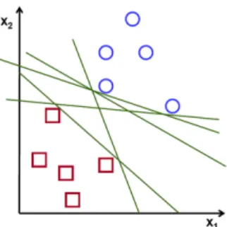
The data for training SVM is a collection of samples that belong to a category (positive samples) and samples that do not belong to the category (negative samples). Each data is represented as a vector in a high-dimensional space. An SVM model determines a hyperplane by which those examples of the separate categories are divided with a clear gap that is as wide as possible. In Figure 3.2, circles and squares represent positive and negative samples respectively. Green lines stand for a separate hyperplanes that can discriminate these two types of samples. Among various separate hyperplanes, SVM selects one so that the margin, a distance between the hyperplane and the closet positive/negative sample, is maximized, as shown in Figure 3.3. Then, new examples are mapped into that same space and predicted to belong to a category based on which side of the hyperplane they fall.

SVM can perform not only linear classification. Using various kernel functions such as Gaus-sian, it can also be used for non-linear classification. At first, we have a plan to try a linear kernel function. If the result is not good as expected, then we will try other kernel functions. In our preliminary experiment, the performance of the linear kernel is the best. Therefore, we train SVM with the linear kernel as the financial classifier.

(23)

Figure 3.2: Support Vector Machine for classification

(24)

Chapter 4 Stock price prediction with FAI

This chapter presents a model to predict future stock prices with our proposed FAI. The goal of training a prediction model is to evaluate ability of FAI for risk management.

4.1 Overview of prediction model

Although many machine learning algorithm can be applicable to train a model to predict stock prices, Long Short-Term Memory (LSTM) [33] is chosen in this study. Because it is well used for prediction of time series.

The structure of LSTM is shown in Figure 4.1[33]. We will introduce basic concepts of LSTM below. First, it has a dynamic “gating" mechanism. Running through the center is the cell state Ii which we interpret as the information flow of the market sensitivity. Second, Ii has a

memory of past time information and more importantly it learns to forget through Figure 4.1. Third, fi is the fraction of past-time information passed over to the present, ˜Ii measures the

information flowing in at the current time and ci is the weight of how important this current

information is.

In our model, input of LSTM is a time sequence of either the stock index, a difference of the stock index, or FAI. The difference of the stock index is defined as a change of the stock index between the current and previous periods. We also train a model where these three kinds of values are passed to the input layer of LSTM. The output of LSTM is a stock index of the next period.

(25)

4.2 Proposed prediction models

In this section, three variations of LSTM for stock price prediction are proposed.

4.2.1 LSTM with single input

The first model uses one type of information as an input. Three kinds of information are considered.

Stock index

The input is a sequence of past stock indexes. Difference of stock index

The input is a sequence of changes of the stock index between succeeding periods. FAI

The input is a sequence of our proposed FAI. As we have already explained, we define a period of LSTM as one transaction day. Note that FAI is calculated for each one week. In this model, the same values is entered during days in a week.

4.2.2 LSTM with multiple inputs

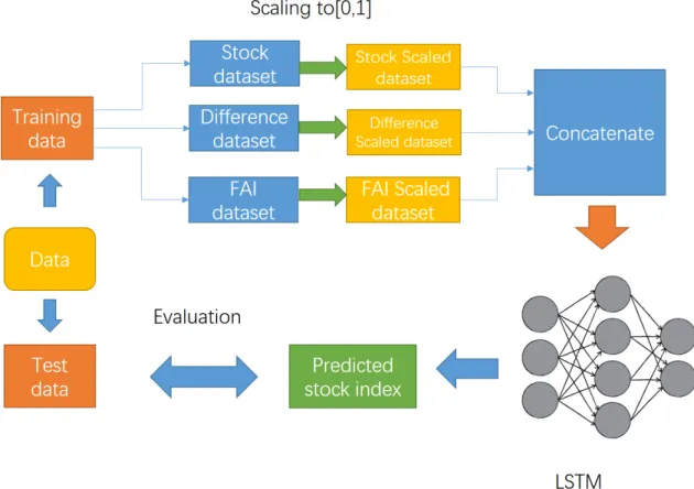
The second model is LSTM that uses three kinds of information explained in Subsection 4.2.1 simultaneously as an input. Values of stock values, difference of stock value, and FAI are concatenated as a vector, then it is passed to the input layer of LSTM. However, the range of these three values are vastly different. A simple concatenation of three values may not be good, since only one type of information that has the greatest absolute value is mainly considered for training LSTM. To tackle this problem, each value is scaled so that all values are in a range between 0 and 1. Scaling is performed in the overall training data. Figure 4.2 illustrates the whole process of training and evaluation of LSTM with multiple inputs.

(26)

Figure 4.2: Overview of LSTM with multiple inputs

4.2.3 Multi-layer LSTM with multiple inputs

Instead of giving a vector of a simple concatenation of three values as an input of LSTM, we consider more sophisticated model of neural network that can accept several inputs. The developer of Keras, a Python library for deep learning, presents a multi-layer neural network with two inputs [4]. The overview of this model is shown in Figure 4.3.

There are two inputs: a main input and an auxiliary input. The main input is used to train the first LSTM(lstm_1) after it is converted to an embedding representation. Then, the output of the lstm_1 is merged with the auxiliary input. Merged data is inputed to a neural network with three hidden layers and one output layer. There are two outputs: a main output and an auxiliary output. The former is the final output of this model, while the latter is the output of lstm_1. The model is trained so that two loss functions of two outputs are minimized. For example, let us consider a task to guess how many retweets and likes a tweet of a new headline obtains. The main input is the news headline, while the auxiliary input is information other than text (e.g. the day when the headline is released). The main output is the guessed number of retweets and likes. The auxiliary output is just used for defining a loss function.

(27)

Figure 4.3: Multi-input and multi-output model of LSTM [4]

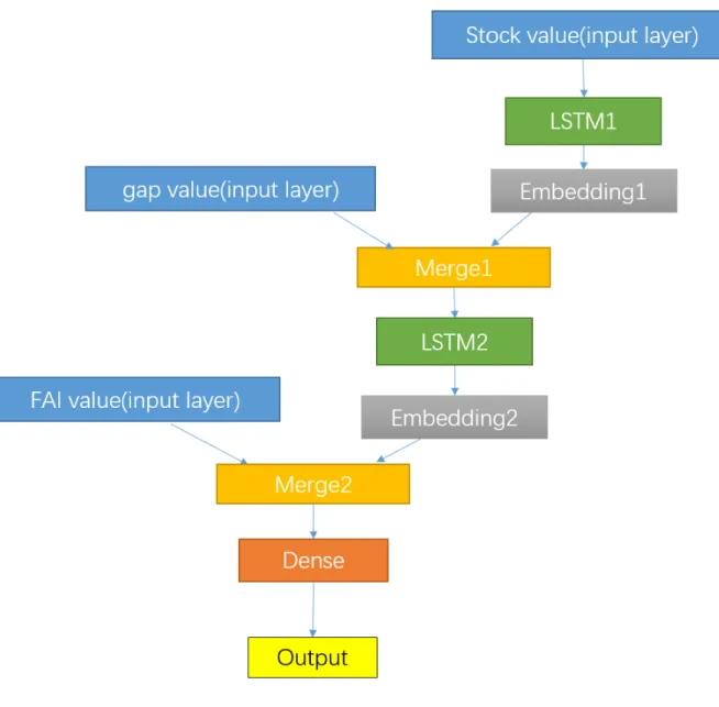
Inspired by the model in Figure 4.3, we design a new multi-layer LSTM model to predict a stock index with three inputs. The overview of our proposed model is shown in Figure 4.4. Since we consider three inputs, two LSTM and one neural network are trained simultaneously. The first input is used to train the first LSTM (LSTM1). The output of LSTM1 is merged with the second input, then it is used for training the second LSTM (LSTM2). Finally, the output of LSTM2 is merged with the third input, then it is passed to the neural network of one hidden layer and one output layer. We define the first, second, and third input as the stock value, the difference of stock values, and FAI, respectively. However, an optimal order of the inputs should be investigated in the future. In our model, the auxiliary outputs are discarded. Two LSTM and neural network have their own loss functions, then the model are trained so that the loss functions are minimized. The algorithm and source code of the layer merging structure design method (multi-layer LSTM multiple inputs model) are shown in Figure A.9 A.10 and A.11 in Appendix A.2.

(28)

(29)

Chapter 5 Evaluation

This chapter reports several experiments to evaluate the effectiveness of our proposed methods. First, Section 5.1 evaluates the performance of financial classifier. Second, Section 5.3 measures correlation between FAI and real stock index. Finally, Section 5.4 evaluates our LSTM-based prediction model with FAI and discuss how well FAI can contribute to avoid financial risks. Before the reports of the second and third experiments, Section 5.2 presents a dataset of stock values that is used for these experiments.

5.1 Classification of financial comment

The classifier to judge whether a comment is related to financial topics, which is described in Section 3.2, takes an import role in FAI. First, the financial classifier is empirically evaluated, and a 10-fold cross validation on our news dataset is carried out. The performance of the classifier is measured by accuracy, which is defined as a ratio of the number of correctly classified comments to the total number of comments.

Table 5.1 shows the accuracy of the two-way and three-way classifiers. Recall that the comments are classified as either “financial-related” or “other”, even when the three-way classifier is used, while both stock-related and related comments are regarded as financial-related comments.

Table 5.1: Result of classification of financial comments

Model Accuracy

Two-way classifier 83.35% Three-way classifier 86.18%

The performance of the financial classifiers is satisfying. We found that the three-way classi-fier outperformed the two-way classiclassi-fier, and, therefore, the three-way classiclassi-fier is used in our step experiments.

5.2 Dataset of stock index

As our FAI is derived from comments of Weibo that is Chinese microblogging service, SSE Composite Index (SCI) is chosen as the stock index in this experiment. SCI is computed from prices of stocks of Chinese companies. It is a tool widely used by investors to describe the market.

(30)

Table 5.2: Result of F -test

Two variables F-test

FAI vs. Stock Index 0.000111

FAI vs. Difference 0.0155

Stock Index vs. Difference 0.00718

The data source of SCI is a finance website of sina1_{. Sina provides us a price at the beginning}

of a day, a price at the end of a day, an average price during a day etc. In this study, the closing price is chosen. We downloaded the closing prices to construct a dataset of stock index. It contains the SCI values of 679 trading days during 28th Oct.2013 to 2nd Aug.2016, which is the same period where the comments on Weibo are downloaded.

5.3 Correlation of financial comment

To evaluate how well FAI can work when used to predict a financial crisis, the correlation between FAI and a real stock index is measured. The F -test, which is a common method for statistical test, is applied FAI values and the real SCI values for 679 trading days in our stock index dataset. We also apply the F -test between FAI and the difference of the stock index as well as the stock index and the difference. Table 5.2 show the results of F -test.

It can be seen that FAI strongly correlates with the stock index, but not with the difference of the stock index. Therefore, it seems difficult to measure the change of the stock index using only FAI.

5.4 Prediction of stock index movement

5.4.1 Goal of experiment

Our stock price prediction method is evaluated in this experiment. Our primary goal is not to get a good return but avoid financial risks. Therefore, the effectiveness of the proposed model is not simply evaluated with respect to how accurate the model can predict the future price. We also discuss how useful the proposed model is to prevent investors from facing a huge loss in financial crisis.

5.4.2 Experimental setting

Our LSTM-based stock index prediction model is evaluated for its ability to predict not the stock index but a movement of the stock index. More precisely, we consider a task to classify a movement of the stock index in one week into one of the following three classes.

Up : This is a case where the stock index goes up by T or more, as shown in (5.1),

Pe− Ps> T. (5.1)

, where Ps and Pe are the stock index at the start and end of the period, respectively.

(31)

Keep : This is a case where the stock index does not change drastically as shown in (5.2),

|Pe− Ps| ≤ T. (5.2)

Down : This is a case where the stock index goes down by T or more, as shown in (5.3),

Pe− Ps< −T. (5.3)

We set T as 0.02 in this experiment.

We have chosen 119 continuous weeks in our stock index dataset to be used as test periods. Usually, for each test period, the data of in the previous days in a fixed length is used for training data as shown in Figure 5.1. In this setting, the amount of the training data is equal to all test periods. Thus the results of test periods can be fairly compared. However, our dataset of SCI index is not large enough to train LSTM. In this experiment, for each test period, all of the past values are used as the training data, as shown in Figure 5.2. Note that more training data is available when the stock movement of the later week is predicted. For the first test period, data of previous 80 transaction days is prepared for training. We chose this experimental setting so that more data can be used for training the LSTM.

Figure 5.1: Common use of test and training data

In order to train LSTM, the number of epochs (the number of iteration of updating parame-ters) should be determined. The procedure to determine it in this experiment is shown below. Recall that there are different training data for 119 weeks in the test data. For each training data, LSTM is trained and a value of the loss function for each epoch is recorded. Figure 5.3 represents an example of change of the loss function against the epochs. The fit function of the library Keras is used to record values of the loss function (or to draw a graph as in Figure 5.3). Keras divides the training data into a reduced training dataset and a development dataset, and outputs values of the loss function in both datasets. We find the minimum number of the epochs where two values of the loss function are converged well. We repeat this procedure for all 119 training data and obtain the number of the epochs at a converged point. Finally, we get the maximum of them. This value is used as the number of the epochs for training LSTM

(32)

Figure 5.2: Use of test and training data in this experiment

in this experiment to repeat iterative learning of parameters until convergence for all training data. Note that not reduced but all training data is used for deep learning in the experiment of the stock price prediction.

Figure 5.3: Change of loss function in terms of epoch

5.4.3 Evaluation criteria

(33)

Accuracy

This is a proportion of the number of the test periods for which the predicted movement class agrees with the true class.

No Lost Accuracy

The main goal of this research is not to help investors get a good return but to help them avoid financial risks. Consequently, it is more important to predict the movement “Down” to avoid making a loss. Therefore, we introduce another criterion, which is called “No Lost Accuracy”. This is the accuracy of the stock movement prediction task where the test periods are classified as either “Down” or not. That is, “Up” and “Keep” classes are merged into one class: “Not-Down”.

5.4.4 Result and discussion

Preliminary evaluation of multi-layer LSTM with multiple inputs

First, a preliminary experiment is conducted to roughly check the performance of our proposed models. As a result, we found that “multi-layer LSTM with multiple inputs” we have explained in Subsection 4.2.3 was not well trained. Its results of the prediction is much worse than expected. Figure 5.4 and 5.5 show the results of the multilayer LSTM with multiple inputs in the first and eighth terms in the test data respectively. Each figure shows the predicted values (orange line) and true values (blue line) for 5 trading days. We can see that the predicted values are the exactly same in both figures. Actually, it is found that the model always predicted the same values for all terms. It is obvious that the model is not trained appropriately at all.

(34)

Figure 5.5: Result of multi-layer LSTM in the eighth term

Although there are several possible reasons why the multi-layer LSTM with multiple inputs can not predict the stock prices correctly, genuine reason seems uncertain. More exploration is required to find problems of this model.

Based on the results of this preliminary experiment, we decided not to evaluate the multi-layer LSTM with multiple inputs in the further experiments.

Performance on overall data

Table 5.3 shows the Accuracy (A) and No Lost Accuracy (NLA) of four different prediction models. Here, “SI”, “DI”, “FAI” stand for the model using only the stock index, the difference of the stock index, and FAI, respectively. “All” stands for the “LSTM with multiple inputs” using three values.

Table 5.3: Results of the stock movement prediction

Model SI DI FAI All

A 31.1% 42.9% 41.2% 35.3%

NLA 47.9% 62.2% 54.6% 57.1%

From these results, it can be seen that “FAI” is better than “SI” in terms of Accuracy and No Lost Accuracy. This indicates that FAI is effective and is able to predict the movement of the stock index. When combining FAI with other indexes, the Not Lost Accuracy is also improved. However, “FAI” does not outperform “DI”. Therefore, it is found that the difference of the stock index is a strong indicator of the movement of the stock market.

Performance on different situations

Figure 5.6 shows a change of SSE Composite Index in our dataset. Every vertical-line represents the highest and lowest stock price in one trading day. Note that the stock prices of only a limited number of days are shown in this graph for simplicity. The red line means the price in a day ended with up, while the green line means it ended with down. Through this graph, we can clearly understand the change of the stock market. In addition, both a bull market and bear market are found in the dataset.

(35)

Figure 5.6: Fluctuation of SCI in dataset

Figure 5.7: Twelve terms of different situations

To evaluate the performance of the prediction models in different situations (bull market, bear market etc.), we divide the test periods into 12 terms, where each term consists of 10 test periods (10 weeks, 50 trading days), and measure the Accuracy and No Lost Accuracy on each term. These twelve terms, T1 ∼ T12, are shown in Figure 5.7. We call the term1(T1) to the term3(T3) as a stage range. We call the term4(T4) to the term(T7) as a bull range. We call the term8(T8) to the term10(10) as a bear range. Again, we also call the term11(T11) to the term12(T12) as a stable range.

(36)

Figure 5.8: Stable range

Figure 5.8 shows the first stable range consisting of three terms. Its time range is from 2013-10-28 to 2014-07-4. The stock index is almost kept stably in this range. The analysis of this range can be compared with bull and bear market.

Figure 5.9: Bull range

Figure 5.9, shows the bull range consisting of four terms. Its time range is from 2014-07-07 to 2015-06-08. We name T4, T5, T6, and T7 as primitive, front, middle, and late bull, respectively. The four bull stages reflect different characteristics of a bull market. T7 is the turning point of the whole market: the trend of market is turned from going up into falling down.

(37)

Figure 5.10: Bear range

Figure 5.10 shows the bear range consisting of three terms. Its time range is from 2015-06-09 to 2016-02-18. We name T8, T9, T10 as front, middle, and late bear, respectively. At the end of the bear market (term 10), the stock index stops falling down, and the stable situation comes back again.

Figure 5.11: stock period table

Figure 5.11, shows the second stable range consisting of two terms. Its time range is from 2016-02-19 to 2016-08-01 .

To evaluate the performance of the prediction models in different situations (bull market, bear market etc.), we divide the test periods into 12 terms, where each term consists of 10 test periods (10 weeks), and we then measure an average of Accuracy and No Lost Accuracy on each term. The results are shown in Table 5.4. The tables include the situation, which is graphically shown in Figure 5.7, for each term.

The results of our experiment show a tendency for the “FAI” model to achieve better per-formance than the other models in both a bull and a bear market. In particular, it is good on a front bull situation (T5). In terms of a bear market (T8, T9, and T10), the “FAI” model is better than or comparable to the others. These results indicate that FAI is effective and it is able to predict a drastic movement of the market. In contrast, the model using the difference of the stock index (DI) works well for stable situations. The model using the stock index (SI) has the worst results in our experiment. Unexpectedly, the “All” model is not always the best choice. Although three values are simply combined as one input vector in our model, this might be a bit too naive.

(38)

Table 5.4: Prediction for different situations (a) Accuracy

Term Situation SI DI FAI All

T1 stable 50% 60% 40% 40% T2 stable 10% 60% 50% 40% T3 stable 30% 40% 40% 20% T4 prim bull 30% 70% 10% 50% T5 front bull 40% 30% 90% 50% T6 mid bull 40% 30% 40% 40% T7 late bull 20% 50% 40% 30% T8 front bear 20% 30% 40% 0% T9 mid bear 10% 40% 30% 50% T10 late bear 40% 20% 50% 10% T11 stable 30% 40% 40% 50% T12 stable 56% 44% 22% 44% (b) No Lost Accuracy

Term Situation SI DI FAI All

T1 stable 70% 60% 50% 70% T2 stable 10% 80% 60% 70% T3 stable 70% 60% 50% 20% T4 prim bull 50% 90% 40% 50% T5 front bull 60% 50% 100% 80% T6 mid bull 50% 50% 50% 70% T7 late bull 30% 60% 40% 50% T8 front bear 40% 50% 50% 50% T9 mid bear 30% 60% 70% 60% T10 late bear 50% 50% 50% 40% T11 stable 50% 70% 50% 70% T12 stable 67% 67% 44% 56%

Comparison between real and predicted index

Figure 5.12: Comparison between SCI predicted by model SI and true SCI (second period) Next, we evaluate how closely the proposed models can predict the stock values. Figure 5.12 shows the stock values predicted by the model SI (orange line) and true stock values (blue line) for the second period in our test data. In this example, the real trend in this term is going up,

(39)

while the predicted trend is falling down. Therefore, it is regarded as failure of prediction when Accuracy and No Lost Accuracy is measured. On the other hand, here we focus on difference between the real and predicted stock values (difference between blue and orange lines). The smaller the difference between them is, the better the trained model is.

The difference between the true and predicted SCI is measured by Mean Squared Error (MSE). It is defined as M SE = 1 N. N X i=1 (pi− ˆpi)2 (5.4)

, where pi and ˆpi are the predicted and true price on the i-th day, and N is the total number

of transaction days in the period.

In Figure 5.12, it shows a predicted result. Both the real Stock Index and predicted values are scalars. The Mean Squared Error(MSE) also reflect the two scalars different distribution. The orange line shows the predicted SCI values, and the blue line shows the real Stock Index trend. In this example, we can know the real trend in this term is going up, but the predicted trend is falling down. So it is not a right predicted result.

(40)

Table 5.5: MSE between real and predicted index (1st-40th periods)

Period Situation SI DI FAI All

p1 stable 0.000067 0.000143 0.006007 0.03501 p2 stable 0.003128 0.000963 0.043082 0.00771 p3 stable 0.000324 0.007941 0.014858 0.0127 p4 stable 0.003003 0.003624 0.031766 0.00144 p5 stable 0.000239 0.001654 0.017111 0.0016 p6 stable 0.000156 0.001912 0.057857 0.00593 p7 stable 0.000295 0.000235 0.035355 0.00325 p8 stable 0.000157 0.002806 0.004947 0.02492 p9 stable 0.000183 0.007352 0.071915 0.02488 p10 stable 0.000056 0.000054 0.060751 0.01081 p11 stable 0.001444 0.000159 0.371546 0.0022 p12 stable 0.000823 0.00046 0.1916 0.00207 p13 stable 0.000565 0.011811 0.050754 0.00079 p14 stable 0.000353 0.000839 0.025183 0.00025 p15 stable 0.000045 0.000151 0.001587 0.00022 p16 stable 0.000464 0.000304 0.023733 0.00495 p17 stable 0.001164 0.001311 0.000734 0.01291 p18 stable 0.001036 0.002245 0.053372 0.00373 p19 stable 0.000125 0.001165 0.025748 0.00445 p20 stable 0.001349 0.000903 0.025819 0.00771 p21 stable 0.000562 0.00503 0.004823 0.0053 p22 stable 0.000252 0.000839 0.11939 0.00253 p23 stable 0.001088 0.001406 0.009592 0.01483 p24 stable 0.000761 0.000615 0.037968 0.03955 p25 stable 0.000141 0.000059 0.037968 0.02671 p26 stable 0.000519 0.00364 0.047385 0.0551 p27 stable 0.00113 0.00508 0.00041 0.0225 p28 stable 0.000198 0.00098 0.8474 0.04364 p29 stable 0.001462 0.000143 0.02594 0.0698 p30 stable 0.000604 0.00029 0.002841 0.05877 p31 prim bull 0.000876 0.001319 0.008138 0.06517 p32 prim bull 0.000189 0.002067 0.13608 0.07435 p33 prim bull 0.000238 0.000609 0.035024 0.08832 p34 prim bull 0.001399 0.023403 0.008308 0.0568 p35 prim bull 0.003466 0.024497 0.004644 0.06075 p36 prim bull 0.0000091 0.008576 0.11969 0.07659 p37 prim bull 0.012404 0.042129 0.00627 0.10468 p38 prim bull 0.000401 0.03647 0.007216 0.05793 p39 prim bull 0.000523 0.107266 0.2132 0.05393 p40 prim bull 0.001338 0.000164 0.076241 0.13781

(41)

p41 front bull 0.003284 0.001259 0.09745 0.15947 p42 front bull 0.006973 0.036387 0.028893 0.180765 p43 front bull 0.005723 0.00411 0.012761 0.20294 p44 front bull 0.000216 0.042307 0.011583 0.36918 p45 front bull 0.002834 0.276406 0.004275 0.437582 p46 front bull 0.000898 0.00667 0.019837 0.49139 p47 front bull 0.002754 0.025857 0.000324 0.57813 p48 front bull 0.002264 0.01077 0.000072 0.48412 p49 front bull 0.000742 0.02807 0.47927 0.42189 p50 front bull 0.001551 0.014263 0.087656 0.33676 p51 mid bull 0.000089 0.087049 0.104085 0.473142 p52 mid bull 0.003261 0.074632 0.07648 0.4285 p53 mid bull 0.000856 0.098112 0.221068 0.46358 p54 mid bull 0.000608 0.067003 0.014153 0.481793 p55 mid bull 0.016209 0.057426 0.168088 0.54086 p56 mid bull 0.000758 0.002002 0.153519 0.771966 p57 mid bull 0.001377 0.034347 0.001628 0.96469 p58 mid bull 0.001362 0.04195 0.021049 0.87049 p59 mid bull 0.006285 0.001614 0.278167 0.916832 p60 mid bull 0.000592 0.00063 0.011655 1.1172 p61 late bull 0.022844 0.007636 0.539664 0.759282 p62 late bull 0.002655 0.001299 0.041588 0.861121 p63 late bull 0.011902 0.002493 8.78 0.771332 p64 late bull 0.004307 0.012507 0.012202 0.9108 p65 late bull 0.015373 0.009751 0.01243 1.24903 p66 late bull 0.002856 0.208229 0.034297 1.44473 p67 late bull 0.001201 0.337428 0.008408 1.102 p68 late bull 0.012613 0.056584 0.003638 0.96272 p69 late bull 0.003033 0.001228 0.047117 0.784173 p70 late bull 0.006178 0.002421 0.000802 0.7029 p71 front bear 0.001651 0.007185 0.001093 0.86005 p72 front bear 0.001052 0.032051 0.033008 0.71967 p73 front bear 0.001273 0.003756 0.051575 0.71679 p74 front bear 0.008744 0.185816 0.001666 0.95284 p75 front bear 0.008079 0.015523 0.037426 0.93806 p76 front bear 0.001297 0.034286 0.014819 0.48822 p77 front bear 0.002475 0.183282 0.14222 0.44541 p78 front bear 0.002469 0.02685 0.002383 0.42642 p79 front bear 0.000564 0.014584 0.009169 0.38363 p80 front bear 0.000531 0.063023 0.005384 0.32555

(42)

p81 mid bear 0.001388 0.000783 0.052966 0.31184 p82 mid bear 0.0009 0.00336 0.014824 0.43025 p83 mid bear 0.00121 0.011635 0.177745 0.53886 p84 mid bear 0.000037 0.001202 0.038596 0.46081 p85 mid bear 0.001087 0.001616 0.002666 0.60606 p86 mid bear 0.002247 0.00089 0.001072 0.62645 p87 mid bear 0.001727 0.002191 2.038315 0.64232 p88 mid bear 0.009695 0.0000959 1.348979 0.65806 p89 mid bear 0.011391 0.017619 0.135546 0.61835 p90 mid bear 0.004717 0.006044 0.001476 0.57532 p91 late bear 0.002625 0.262025 0.003813 0.61427 p92 late bear 0.011644 0.008597 0.026467 0.80151 p93 late bear 0.000196 0.002041 0.831589 0.70742 p94 late bear 0.001289 0.006381 0.001003 0.49182 p95 late bear 0.008815 1.182078 0.187348 0.45676 p96 late bear 0.002125 0.02696 0.187348 0.45676 p97 late bear 0.002125 0.02696 9.097692 0.31755 p98 late bear 0.000162 0.001051 3.7557 0.197 p99 late bear 0.001107 0.01943 0.002799 0.22932 p100 late bear 0.002559 0.000454 0.040563 0.13613 p101 stable 0.001441 0.001373 0.082176 0.16884 p102 stable 0.000269 0.001195 0.033125 0.13018 p103 stable 0.001233 0.014162 0.022594 0.23608 p104 stable 0.001944 0.000397 0.051551 0.2192 p105 stable 0.000091 0.000138 0.6351 0.2798 p106 stable 0.000366 0.041001 0.021458 0.3172 p107 stable 0.000166 0.002334 0.05018 0.3139 p108 stable 0.000493 0.000771 0.0353 0.25271 p109 stable 0.00109 0.000125 0.56728 0.28427 p110 stable 0.000602 0.000043 0.216294 0.19025 p111 stable 0.000198 0.000787 0.000821 0.16563 p112 stable 0.000139 0.001655 0.976874 0.119 p113 stable 0.00022 0.076248 0.036548 0.18021 p114 stable 0.001231 0.00639 0.566031 0.21706 p115 stable 0.0000053 0.007126 0.011652 0.18174 p116 stable 0.001779 0.008203 0.017394 0.15743 p117 stable 0.00051 0.000631 0.34216 0.20407 p118 stable 0.00081 0.001533 6.88079 0.23814 p119 stable 0.000253 0.00144 0.04704 0.32023

(43)

Table 5.8: Average of MSE

Model SI DI FAI All

stable 0.0006781 0.004687 0.2619 0.09556

bull 0.004063 0.04492 0.2972 0.5254

bear 0.003143 0.07133 0.6959 0.5277

overall 0.002437 0.03501 0.3777 0.3489

Table 5.8 reveals the macro average of MSE for stable situation, bull situation, bear situation and overall periods. As reported earlier, “stable” terms are T1, T2, T3, T11, and T12; “bull” terms are T4, T5, T6, and T7; “bear” terms are T8, T9, and T10. First, no matter which period, MSE of SI is the best (smallest), and MSE of DI is the second best. MSE of FAI and ALL is much greater than that of SI and DI. Comparing FAI and ALL, FAI is better than ALL in only bull period. These results indicate that the stock values predicted by the model using FAI are far from the real values. However, even when the stock index cannot be predicted closely, it is fine to predict the movement of stock index correctly. To avoid a financial risk, prediction of a drastic change is more important. Let us consider the example in Figure 5.13. In this figure, although the model FAI cannot predict the exact values of SCI, it can correctly predict that the market is going down.

(44)

Chapter 6 Conclusion

6.1 Summary

This paper investigates whether the financial attention of investors as measured from a large collection of comments on Weibo could predict a down occasion on the SSE Composite In-dex(SCI). The FAI is defined as a proportion of the financial related comments and estimated by the financial classifier trained from the news articles. The FAI, in addition to the stock index and the difference of the index were used as the input of the LSTM model to predict the future stock index.

The results of our experiment showed that the accuracy of the LSTM with FAI was better than the model with the difference of the stock index on average but it was better or comparable in bear markets. Therefore, the FAI could be an effective index to predict a financial risk and this can help investors to avoid making a massive loss. In addition, the FAI could also effectively predict the beginning of a bull market because the prediction model with FAI worked well in a front bull term. That is, the FAI can be use to detect turning points in a stock market, no matter if prices move down or up.

In this thesis, we did not only used a well-known effective prediction model, i.e. LSTM, but also tried to design the new architecture of LSTM that accepted multiple types of inputs. How to design structure of neural networks to handle multiple inputs is still an important open question. The simple way where multiple inputs were just concatenated as a single vector was tried first. We also proposed a cascaded LSTM where three kinds of indexes are given one by one. Since the results of the new model were not good as expected, how to combine the stock value and FAI for prediction of stock prices should be carefully investigated in the future.

6.2 Future work

Although the results of the experiments have proven the effectiveness of our proposed method, there is still room for improvement. Given that the number of SNS comments might be in-sufficient, we plan to get more comments from Weibo to improve the quality of the FAI. As discussed in the previous section, the way to incorporate three kinds of information into LSTM for stock price prediction should be thoroughly investigated. In addition, it would be worth to try to find other useful information for prediction of financial crisis.

As for the implementation of LSTM, we used Keras tool to develop our prediction model of stock index, since it is one of the best libraries for deep learning. However, the disadvantages of Keras is from its top design model, which limits the basic deep learning function. Instead, we will use other public libraries for deep learning such as Tensorflow or Pytorch for training our proposed LSTM and check how the performance of prediction can be improved.

(45)

Finally, in our experiment, Weibo is used as SNS for calculating FAI and the stock index in Chinese market (SCI) is used as the target index to be predicted. However, Chinese stock market is still in a developing stage. For example, laws and rules on the Chinese stock market are not prepared well. Therefore, the ability of FAI to foresee financial crisis should be verified against several stock markets of other countries including more mature ones..

JAIST Repository: Measuring Financial Crisis Index for Risk Warning through Analysis of Social Network