The Impact of Mislabelling on the Performance and Interpretation of Defect Prediction Models

全文

(1)奈良先端科学技術⼤学院⼤学学術リポジトリ Nara Institute of Science and Technology Academic Repository: naistar. Title. Author(s). Citation. The Impact of Mislabelling on the Performance and Interpretation of Defect Prediction Models Tantithamthavorn, Chakkrit; McIntosh, Shane; Hassan, Ahmed E.; Ihara, Akinori; Matsumoto, Kenichi 2015 IEEE/ACM 37th IEEE International Conference on Software Engineering, 6-24 May 2015, Florence, Italy. Issue Date. 2015. Resource Version. author © 2015 IEEE. Personal use of this material is permitted. Permission from IEEE must be obtained for all other uses, in any current or future media,. Rights. including reprinting/republishing this material for advertising or promotional purposes, creating new collective works, for resale or redistribution to servers or lists, or reuse of any copyrighted component of this work in other works.. DOI. 10.1109/ICSE.2015.93. URL. http://hdl.handle.net/10061/12736.

(2) The Impact of Mislabelling on the Performance and Interpretation of Defect Prediction Models Chakkrit Tantithamthavorn† , Shane McIntosh‡ , Ahmed E. Hassan‡ , Akinori Ihara† , Ken-ichi Matsumoto† † Graduate. School of Information Science, Nara Institute of Science and Technology, Japan. {chakkrit-t,akinori-i,matumoto}@is.naist.jp ‡ School of Computing, Queen’s University, Canada. {mcintosh,ahmed}@cs.queensu.ca. Abstract—The reliability of a prediction model depends on the quality of the data from which it was trained. Therefore, defect prediction models may be unreliable if they are trained using noisy data. Recent research suggests that randomly-injected noise that changes the classification (label) of software modules from defective to clean (and vice versa) can impact the performance of defect models. Yet, in reality, incorrectly labelled (i.e., mislabelled) issue reports are likely non-random. In this paper, we study whether mislabelling is random, and the impact that realistic mislabelling has on the performance and interpretation of defect models. Through a case study of 3,931 manually-curated issue reports from the Apache Jackrabbit and Lucene systems, we find that: (1) issue report mislabelling is not random; (2) precision is rarely impacted by mislabelled issue reports, suggesting that practitioners can rely on the accuracy of modules labelled as defective by models that are trained using noisy data; (3) however, models trained on noisy data typically achieve 56%-68% of the recall of models trained on clean data; and (4) only the metrics in top influence rank of our defect models are robust to the noise introduced by mislabelling, suggesting that the less influential metrics of models that are trained on noisy data should not be interpreted or used to make decisions.. I. I NTRODUCTION Defect models, which identify defect-prone software modules using a variety of software metrics [15, 39, 45], serve two main purposes. First, defect models can be used to predict [1, 11, 17, 27, 33, 34, 36, 42, 51] modules that are likely to be defect-prone. Software Quality Assurance (SQA) teams can use defect models in a prediction setting to effectively allocate their limited resources to the modules that are most likely to be defective. Second, defect models can be used to understand [10, 30, 32, 33, 46, 47] the impact that various software metrics have on the defect-proneness of a module. The insights derived from defect models can help software teams to avoid pitfalls that have often led to defective software modules in the past. The accuracy of the predictions and insights derived from defect models depends on the quality of the data from which these models are trained. Indeed, Mockus argues that poor data quality can lead to biased conclusions [31]. Defect models are trained using datasets that connect issue reports recorded in an Issue Tracking System (ITS) with the software modules that are impacted by the associated code changes that address these issue reports. The code changes are in turn recorded in a Version Control System (VCS). Thus, the quality of the data recorded in the ITS and VCS impacts the quality of the data. used to train defect models [2, 5, 6, 19, 37]. Recent research shows that the noise that is generated by issue report mislabelling, i.e., issue reports that describe defects but were not classified as such (or vice versa), may impact the performance of defect models [26, 41]. Yet, while issue report mislabelling is likely influenced by characteristics of the issue itself — e.g., novice developers may be more likely to mislabel an issue than an experienced developer — the prior work randomly generates mislabelled issues. In this paper, we set out to investigate whether mislabelled issue reports can be accurately explained using characteristics of the issue reports themselves, and what impact a realistic amount of noise has on the predictions and insights derived from defect models. Using the manually-curated dataset of mislabelled issue reports provided by Herzig et al. [19], we generate three types of defect datasets: (1) realistic noisy datasets that contain mislabelled issue reports as classified manually by Herzig et al., (2) random noisy datasets that contain the same proportion of mislabelled issue reports as contained in the realistic noisy dataset, however the mislabelled issue reports are selected at random, and (3) clean datasets that contain no mislabelled issues (we use Herzig et al.’s data to reassign the mislabelled issue reports to their correct categories). Through a case study of 3,931 issue reports spread across 22 releases of the Apache Jackrabbit and Lucene systems, we address the following three research questions: (RQ1) Is mislabelling truly random? Issue report mislabelling is not random. Our models can predict mislabelled issue reports with a mean Fmeasure that is 4-34 times better than that of random guessing. The tendency of a reporter to mislabel issues in the past is consistently the most influential metric used by our models. (RQ2) How does mislabelling impact the performance of defect models? We find that the precision of our defect models is rarely impacted by mislabelling. Hence, practitioners can rely on the accuracy of modules labelled as defective by defect models that are trained using noisy data. However, cleaning the data prior to training the defect models will likely improve their ability to identify all defective modules..

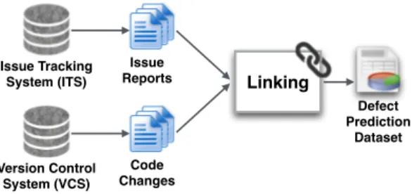
(3) (RQ3) How does mislabelling impact the interpretation of defect models? We find that 80%-85% of the metrics in the top influence rank of the clean models also appear in the top influence rank of the noisy models, indicating that the most influential metrics are not heavily impacted by issue report mislabelling. On the other hand, as little as 18% of the metrics in the second and third influence rank of the clean models appear in the same rank in the noisy models, which suggests that the less influential metrics are more unstable. Furthermore, we find that randomly injecting mislabelled defects tends to overestimate the impact that mislabelling truly has on model performance and model interpretation. Paper organization. The remainder of this paper is organized as follows. Section II situates this paper with respect to the related work. Section III discusses the design of our case study, while Section IV presents the results with respect to our three research questions. Section V discloses the threats to the validity of our work. Finally, Section VI draws conclusions. II. R ELATED W ORK & R ESEARCH Q UESTIONS Given a software module, such as a source code file, a defect model classifies it as either likely to be defective or clean. Defect models do so by modelling the relationship between module metrics (e.g., size and complexity), and module class (defective or clean). As shown in Figure 1, module metrics and classes are typically mined from historical repositories, such as ITSs and VCSs. First, issue reports, which describe defects, feature requests, and general maintenance tasks, are extracted from the ITS. Next, the historical code changes that are recorded in a VCS are extracted. Finally, these issue reports are linked to the code changes that have been performed in order to address them. For example, a module’s class is set to defective if it has been affected by a code change that addresses an issue report that is classified as a defect. Various data quality issues can arise when constructing defect prediction datasets. Specifically, prior work has investigated data quality issues with respect to the linkage process and the issue reports themselves. We describe the prior work with respect to each data quality issue below. A. Linkage of Issue Reports with Code Changes The process of linking issue reports with code changes can generate noise in defect prediction datasets, since the linkage process often depends on manually-entered links that are provided by developers. Bachmann et al. find that the issue reports of several defects are not identified in the commit logs [5], and thus are not visible to the automated linking tools that are used to extract defect datasets. Wu et al. [50] and Nguyen et al. [37] use the textual similarity between issue reports and version control logs to recover the missing links between the ITS and VCS repositories.. Issue Tracking System (ITS). Issue Reports. Linking Defect Prediction Dataset. Version Control System (VCS). Code Changes. Fig. 1: The construction of defect prediction datasets.. The noise generated by missing links in defect prediction datasets introduces bias. Bird et al. find that more experienced developers are more likely to explicitly link issue reports to the corresponding code changes [6]. Nguyen et al. find that such biases also exist in commercial datasets [38], which were suspected to be “near-ideal.” Rahman et al. examined the impact of bias on defect models by generating artificially biased datasets [40], reporting that the size of the generated dataset matters more than the amount of injected bias. Linkage noise and bias are addressed by modern tools like JIRA1 and IBM Jazz2 that automatically link issue reports with code changes. Nevertheless, recent work by Nguyen et al. shows that even when such modern tools are used, bias still creeps into defect datasets [38]. Hence, techniques are needed to detect and cope with biases in defect prediction datasets. B. Mislabelled Issue Reports Even if all of the links between issue reports and code changes are correctly recovered, noise may creep into defect prediction datasets if the issue reports themselves are mislabelled. Aranda and Venolia find that ITS and VCS repositories are noisy sources of data [3]. Antoniol et al. find that textual features can be used to classify issue reports [2], e.g., the term “crash” is more often used in the issue reports of defects than other types of issue reports. Herzig et al. find that 43% of all issue reports are mislabelled, and this mislabelling impacts the ranking of the most defect-prone files [19]. Mislabelled issue reports generate noise that impacts defect prediction models. Yet, little is known about the nature of mislabelling. For example, do mislabelled issue reports truly appear at random throughout defect prediction datasets, or are they explainable using characteristics of code changes and issue reports? Knowledge of the characteristics that lead to mislabelling would help researchers to more effectively filter (or repair) mislabelled issue reports in defect prediction datasets. Hence, we formulate the following research question: (RQ1) Is mislabelling truly random? Prior work has shown that issue report mislabelling may impact the performance of defect models. Kim et al. find 1 https://issues.apache.org/jira/ 2 http://www.jazz.net/.

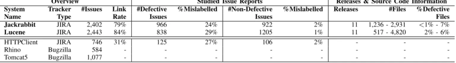
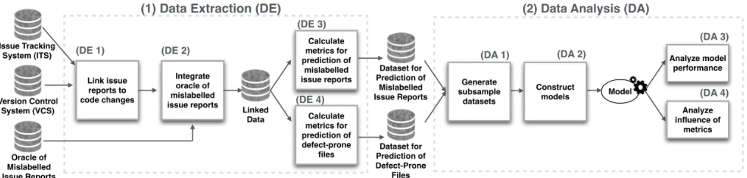
(4) TABLE I: An overview of the studied systems. Those above the double line satisfy our criteria for analysis. System Name Jackrabbit Lucene HTTPClient Rhino Tomcat5. Overview Tracker #Issues Type JIRA 2,402 JIRA 2,443 JIRA 746 Bugzilla 584 Bugzilla 1,077. Link Rate 79% 84% 31% -. #Defective Issues 966 838 125 -. Studied Issue Reports %Mislabelled #Non-Defective Issues 24% 922 29% 1205 27% 106 -. that defect models are considerably less accurate when they are trained using datasets that have a 20%-35% mislabelling rate [26]. Seiffert et al. conduct a comprehensive study [44], and the results confirm the prior findings of Kim et al. [26]. However, prior work assumes that issue report mislabelling is random, which is not necessarily true. For example, novice developers may be more likely to mislabel an issue report than experienced developers. Hence, we set out to address the following research question: (RQ2) How does mislabelling impact the performance of defect models? In addition to being used for prediction, defect models are also used to understand the characteristics of defectprone modules. Mockus et al. study the relationship between developer-centric measures of organizational change and the probability of customer-reported defects in the context of a large software system [32]. Cataldo et al. study the impact of software and work dependencies on software quality [10]. Shihab et al. study the characteristics of high-impact and surprise defects [47]. McIntosh et al. study the relationship between software quality and modern code review practices [30]. Such an understanding of defect-proneness is essential to chart quality improvement plans. Mislabelled issue reports likely impact the interpretation of defect models as well. To investigate this, we formulate the following research question: (RQ3) How does mislabelling impact the interpretation of defect models?. III. C ASE S TUDY D ESIGN In this section, we outline our criteria for selecting the studied systems, and our data extraction and analysis approaches. A. Studied Systems To address our research questions, we need a dataset of mislabelled issue reports. In selecting the studied systems, we identified two important criteria that needed to be satisfied: – Criterion 1 — Mislabelled issue report oracle: In order to study the impact that mislabelling has on defect prediction models, we need an oracle of which issues have been mislabelled.. %Mislabelled 2% 1% 2% -. Releases & Source Code Information Releases #Files %Defective Files 11 1,236 - 2,931 <1% - 7% 11 517 - 4,820 2% - 6% -. – Criterion 2 — Issue report linking rate: The issue reports for each studied system must be traceable, i.e., an issue report must establish a link to the code change that addresses it. Systems with low rates of traceable issue reports will introduce too many missing links [5, 6], which may impact the performance of our defect models [40]. Hence, we only study systems where a large proportion of issue reports can be mapped to the code changes that address them. To satisfy criterion 1, we began our study using the corpus of mislabelled issue reports that was manually-curated by Herzig et al. [20]. Table I provides an overview of the five systems in the corpus. To satisfy criterion 2, we first select the set of systems in the corpus of Herzig et al. that use the JIRA ITS.1 JIRA explicitly links code changes to the issue reports that they address. Since Rhino and Tomcat5 do not use JIRA, we removed them from our analysis. Next, we discard systems that do not have a high linkage rate. We discard HTTPClient, since fewer than half of the issue reports could be linked to the code changes that address them. Table I shows that the Jackrabbit and Lucene systems satisfied our criteria for analysis. Jackrabbit is a digital content repository that stores versioned entries in a hierarchy.3 Lucene is a library offering common search indexing functionality.4 B. Data Extraction In order to produce the datasets necessary for our study, we first need to extract data from the ITS of each studied system. Next, we need to link the extracted ITS data with entries from the respective VCS repositories, as well as with the oracle of mislabelled issue reports. Figure 2 provides an overview of our data extraction approach, which is further divided into the four steps that we describe below. (DE 1) Link issue reports to code changes. We first extract the issue reports from the ITS of each studied system. Then, we extract the references to code changes from those issue reports. Finally, we extract the commit information for the referenced code changes from the VCS. (DE 2) Integrate oracle of mislabelled issue reports. We link the oracle of mislabelled issue reports with our defect datasets for two purposes. First, we record the mislabelled issues in order to train models that predict and explain the nature of mislabelling (cf. RQ1). Second, we use the oracle to 3 http://jackrabbit.apache.org/ 4 http://lucene.apache.org/.

(5) (1) Data Extraction (DE). (2) Data Analysis (DA) (DE 3). Issue Tracking System (ITS). Version Control System (VCS). (DE 1) Link issue reports to code changes. Calculate metrics for prediction of mislabelled issue reports. (DE 2) Integrate oracle of mislabelled issue reports. Oracle of Mislabelled Issue Reports. (DE 4) Linked Data. Calculate metrics for prediction of defect-prone ﬁles. (DA 3) (DA 2). (DA 1) Dataset for Prediction of Mislabelled Issue Reports. Generate subsample datasets. Construct models. Analyze model performance Model. (DA 4) Analyze inﬂuence of metrics. Dataset for Prediction of Defect-Prone Files. Fig. 2: An overview of our data extraction and analysis approaches. TABLE II: Factors used to study the nature of mislabelled issue reports (RQ1). Metrics Diffusion Dimension # Files, # Components, # Subsystems Entropy Size Dimension # Commits Churn. History Dimension Reporter tendency Code tendency. Communication Dimension Discussion length. Description The number of unique files, components, and subsystems that are involved in the code changes that address an issue report. The dispersion of a change across the involved files. The number of commits made to address an issue report. The sum of the added and removed lines in the code changes made to address an issue report. The proportion of prior issue reports that were previously filed by the reporter of this issue and that were mislabelled. For each file involved in the code changes that address an issue report, we calculate the proportion of its prior issue reports that were mislabelled. For each issue report, we select the maximum of the proportions of each of its files.. TABLE III: The factors that we use to build our defect models (RQ2, RQ3). Metrics Process Metrics # Commits. Description. Normalized added. lines. Normalized deleted. lines. Churn Developer Metrics Active developer Distinct developer Minor contributor Ownership Metrics Ownership ratio Owner experience. The number of comments that were posted on the issue report. Committer experience. correct mislabelled issues in order to produce clean (mislabelfree) versions of our defect prediction datasets. We use this data to study the impact of mislabelling on the performance and interpretation of our models (cf. RQ2 and RQ3). (DE 3) Calculate metrics for the prediction of mislabelled issue reports. In order to address RQ1, we train models that classify whether an issue report is mislabelled or not. Table II shows the nine metrics that we use to predict whether an issue report is mislabelled or not. These nine metrics capture four dimensions of an issue report that we briefly describe below. Diffusion metrics measure the dispersion of a change across modules. Since broadly-dispersed code changes may contain several different concepts, they are likely difficult to accurately label. We use four metrics to measure diffusion as described below. The # Subsystems, # Components, and # Files metrics measure the spread of a change at different granularities. For example, for a file org/apache/lucene/index/values/Reader.java,. Number of commits made to a file during a studied release. Number of added lines in this file normalized by the sum of all lines added to all files during a studied release. Number of deleted lines in this file normalized by the sum of all lines deleted from all files during a studied release. The sum of added and removed lines in a file during a studied release. Number of developers who made a change to a file during a studied release. Number of distinct developers who made a change to a file during or prior to a studied release. Number of developers who have authored less than 5% of the changes to a file. The propotion of lines written by the author who made the most changes to a file. The experience (i.e., the proportion of all of the lines in a project that have been written by an author) of the most active contributor to a file. The geometric mean of the experiences of all of the developers that contributed to a file.. the subsystem is org.apache.lucene.index and the component is org/apache/lucene/index/values. We count the number of unique subsystems, components, and files that are modified by a change by analyzing the file paths as described above. We also measure the entropy (i.e., disorder) of a change. We use the entropy definition of prior work Pn[17, 23], i.e., the entropy of a change C is H(C) = − k=1 (pk × log2 pk ), where N is the number of files included in a change, pk is the proportion of change C that impacts file k. The larger the entropy value, the more broadly that a change is dispersed among files. Size metrics measure how much code change was required to address an issue report. Similar to diffusion, we suspect that larger changes may contain more concepts, which likely makes the task of labelling more difficult. We measure the size of a change by the # commits (i.e., the number of changes in the VCS history that are related to this issue report) and the.

(6) churn (i.e., the sum of the added and removed lines). History metrics measure the tendency of files and reporters to be involved with mislabelled issue reports. Files and reporters that have often been involved with mislabelled issue reports in the past are likely to be involved with mislabelled issue reports in the future. The reporter tendency is the proportion of prior issue reports that were created by a given reporter and were mislabelled. To calculate the code tendency for an issue report r, we first compute the tendency of mislabelling for each involved file fk , i.e., the proportion of prior issue reports that involve fk that were mislabelled. We select the maximum of the mislabelling tendencies of fk to represent r. Communication metrics measure the degree of discussion that occurred on an issue report. Issue reports that are discussed more are likely better understood, and hence are less likely to be mislabelled. We represent the communication dimension with the discussion length metric, which counts the number of comments posted on an issue report. (DE 4) Calculate metrics for the prediction of defect-prone files. In order to address RQ2 and RQ3, we train defect models that identify defect-prone files. Table III shows the ten metrics that are spread across three dimensions that we use to predict defect-prone files. These metrics have been used in several previous defect prediction studies [4, 7, 24, 33– 35, 40, 46, 49]. We briefly describe each dimension below. Process metrics measure the change activity of a file. We count the number of commits, lines added, lines deleted, and churn to measure change activity of each file. Similar to Rahman et al. [40], we normalize the lines added and lines deleted of a file by the total lines added and lines deleted. Developer metrics measure the size of the team involved in the development of each file [7]. Active developers counts the developers who have made changes to a file during the studied release period. Distinct developers counts the developers who have made changes to a file up to (and including) the studied release period. Minor developers counts the number of developers who have authored less than 5% of the changes to a file in the studied release period. Ownership metrics measure how much of the change to a file has been contributed by a single author [7]. Ownership ratio is the proportion of the changed lines to a file that have been contributed by the most active author. We measure the experience of an author using the proportion of changed lines in all of the system files that have been contributed by that author. Owner experience is the experience of the most active author of a file. Committer experience is the geometric mean of the experiences of the authors that contributed to a file. C. Data Analysis We train models using the datasets that we extracted from each studied system. We then analyze the performance of these models, and measure the influence that each of our metrics has on model predictions. Figure 2 provides an overview of our data analysis approach, which is divided into four steps. We describe each step below.. (DA 1) Generate bootstrap datasets. In order to ensure that the conclusions that we draw about our models are robust, we use the bootstrap resampling technique [12]. The bootstrap randomly samples K observations with replacement from the original dataset of size K. Using the bootstrap technique, we repeat our experiments several times, i.e., once for each bootstrap sample. We use implementation of the bootstrap algorithm provided by the boot R package [9]. Unlike k-fold cross-validation, the bootstrap technique fits models using the entire dataset. Cross-validation splits the data into k equal parts, using k - 1 parts for fitting the model, setting aside 1 fold for testing. The process is repeated k times, using a different part for testing each time. Notice, however, that models are fit using k - 1 folds (i.e., a subset) of the dataset. Models fit using the full dataset are not directly tested when using k-fold cross-validation. Previous research demonstrates that the bootstrap leads to considerably more stable results for unseen data points [12, 16]. Moreover, the use of bootstrap is recommended for high-skewed datasets [16], as is the case in our defect prediction datasets. (DA 2) Construct models. We train our models using the random forest classification technique [8]. Random forest is an accurate classification technique that is robust to noisy data [22, 48], and has been used in several previous studies [13, 14, 22, 24, 28]. The random forest technique constructs a large number of decision trees at training time. Each node in a decision tree is split using a random subset of all of the metrics. Performing this random split ensures that all of the trees have a low correlation between them. Since each tree in the forest may report a different outcome, the final class of a work item is decided by aggregating the votes from all trees and deciding whether the final score is higher than a chosen threshold. We use the implementation of the random forest technique provided by the bigrf R package [29]. We use the approach described by Harrell Jr. to train and test our models using the bootstrap and original samples [16]. In theory, the relationship between the bootstrap samples and the original data is asymptotically equivalent to the relationship between the original data and its population [16]. Since the population of our datasets is unknown, we cannot train a model on the original dataset and test it on the population. Hence, we use the bootstrap samples to approximate this by using several thousand bootstrap samples to train several models, and test each of them using the original data. Handling skewed metrics: Analysis of the distributions of our metrics reveals that they are right-skewed. To mitigate this skew, we log-transform each metric prior to training our models (ln(x + 1)). Handling redundant metrics: Correlation analysis reduces collinearity among our metrics, however it would not detect all of the redundant metrics, i.e., metrics that do not have a unique signal with respect to the other metrics. Redundant metrics will interfere with each other, distorting the modelled relationship between the module metrics and its class. We, therefore, remove redundant metrics prior to constructing our defect models. In order to detect redundant metrics, we fit.

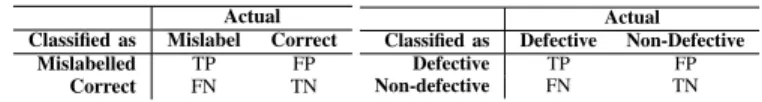
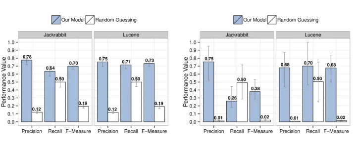
(7) Classified as Mislabelled Correct. Actual Mislabel Correct TP FP FN TN. Classified as Defective Non-defective. Defective TP FN. Actual Non-Defective FP TN. (a) Prediction of mislabelled is- (b) Prediction of defect-prone files. sue reports. TABLE IV: Example confusion matrices.. preliminary models that explain each metric using the other metrics. We use the R2 value of the preliminary models to measure how well each metric is explained by the others. We use the implementation of this approach provided by the redun function of the rms R package. The function builds preliminary models for each metric for each bootstrap iteration. The metric that is most well-explained by the other metrics is iteratively dropped until either: (1) no preliminary model achieves an R2 above a cutoff threshold (for this paper, we use the default threshold of 0.9), or (2) removing a metric would make a previously dropped metric no longer explainable, i.e., its preliminary model will no longer achieve an R2 exceeding our 0.9 threshold. Handling imbalanced categories: Table I shows that our dependent variables are imbalanced, e.g., there are more correctly labelled issue reports than mislabelled ones. If left untreated, the models trained using imbalanced data will favour the majority category, since it offers more predictive power. In our case, the models will more accurately identify correctlylabelled issue reports than mislabelled ones. To combat the bias of imbalanced categories, we re-balance the training corpus to improve the performance of the minority category. We re-balance the data using a re-sampling technique that removes samples from the majority category (undersampling) and repeats samples in the minority category (oversampling). We only apply re-balancing to bootstrap samples (training data) — the original (testing) data is not re-balanced. (DA 3) Analyze model performance. To evaluate the performance of the prediction models, we use the traditional evaluation metrics in defect prediction, i.e., precision, recall, and F-measure. These metrics are calculated using the confusion matrices of Table IV. Precision measures the proportion of TP classified entities that are correct ( TP+FP ). Recall measures the TP ). F-measure proportion of correctly classified entities ( TP+FN is the harmonic mean of precision and recall ( 2×Precision×Recall Precision+Recall ). (DA 4) Analyze influence of metrics. To study the most influential metrics in our random forest models, we compute Breiman’s variable importance score [8] for each studied metric. The larger the score, the greater the influence of the metric on our models. We use the varimp function of the bigrf R package [29] to compute the variable importance scores of our metrics. To study the influence that the studied metrics have on our models, we apply the Scott-Knott test [43]. Each metric will have several variable importance scores (i.e., one from each of the releases). The Scott-Knott test will cluster the metrics according to statistically significant differences in their mean ranks (α = 0.05). We use the implementation of the Scott-. Knott test provided by the ScottKnott R package [21]. The Scott-Knott test ranks each metric exactly once, however several metrics may appear within one rank. IV. C ASE S TUDY R ESULTS In this section, we present the results of our case study with respect to our three research questions. (RQ1) Is mislabelling truly random? To address RQ1, we train models that indicate whether or not an issue report was mislabelled. We build two types of mislabelling models — one to predict issue reports that were incorrectly labelled as defects (defect mislabelling, i.e., false positives), and another to predict issue reports that should have been labelled as defects, but were not (non-defect mislabelling, i.e., false negatives). We then measure the performance of these models (RQ1-a) and study the impact of each of our issue report metrics in Table II (RQ1-b). (RQ1-a) Model performance. Figure 3 shows the performance of 1,000 bootstrap-trained models. The error bars indicate the 95% confidence interval of the performance of the bootstrap-trained models, while the height of the bars indicates the mean performance of these models. We compare the performance of our models to random guessing. Our models achieve a mean F-measure of 0.38-0.73, which is 4-34 times better than random guessing. Figure 3 also shows that our models also achieve a mean precision of 0.68-0.78, which is 6-75 times better than random guessing. Due to the scarcity of non-defect mislabelling (see Table I), we observe broader ranges covered by the confidence intervals of the performance values in Figure 3b. Nonetheless, the ranges covered by the confidence intervals of the precision and F-measure of all of our models does not overlap with those of random guessing. Given the skewed nature of the distributions at hand, we opt to use a bootstrap t-test, which is distribution independent. The results show that the differences are statistically significant (α = 0.05). Figure 3b shows that the only case where our models underperform with respect to random guessing is the non-defect mislabelling model on the Jackrabbit system. Although the mean recall of our model is lower in this case, the mean precision and F-measure are still much higher than that of random guessing. (RQ1-b) Influence of metrics. We calculate the variable importance scores of our metrics in 1,000 bootstrap-trained models, and cluster the results using the Scott-Knott test. A reporter’s tendency to mislabel issues in the past is the most influential metric for predicting mislabelled issue reports. We find that reporter tendency is the only metric in the top Scott-Knott cluster, indicating that it is consistently the most influential metric for our mislabelling models. Moreover, for defect mislabelling, reporter tendency is the most influential metric in 94% of our bootstrapped Jackrabbit models and 86% of our Lucene models. Similar to RQ1-a, we find that there is more variability in the influential metrics of our non-defect mislabelling models than.

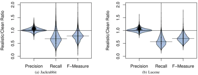
(8) Our Model. Random Guessing. Jackrabbit. Our Model. Lucene. Jackrabbit. 1.0 0.75. 0.73. 0.71. 0.70 0.64. 0.6 0.50. 0.5. 0.50. 0.4 0.3 0.19 0.12. 0.19 0.12. Performance Value. Performance Value. 0.9 0.78. 0.7. 0.2. Lucene. 1.0. 0.9 0.8. Random Guessing. 0.8. 0.38. 0.4 0.3. 0.26. 0.2 0.1 0.0. Precision. 0.68 0.50. 0.50. 0.5. 0.0 Recall F−Measure. 0.70. 0.68. 0.6. 0.1. Precision. 0.75. 0.7. Recall F−Measure. 0.02. 0.01. Precision. (a) Defect mislabelling (false positive). Recall F−Measure. 0.02. 0.01. Precision. Recall F−Measure. (b) Non-defect mislabelling (false negative). Fig. 3: A comparison of the performance of our models that are trained to identify mislabelled issue reports (blue) against random guessing (white). Error bars indicate the 95% confidence interval based on 1,000 bootstrap iterations.. Clean Data. Repeat 1,000 times Bootstrap Sample. (Step 2). (Step 3). Analyze models. Model Realistically Realistic Noisy Sample. 0.5. 1.0. Model Clean Sample. 0.0. Issue report mislabelling is not random. Our models can predict mislabelled issue reports with a mean F-measure that is 4-34 times better than that of random guessing. The tendency of a reporter to mislabel issues in the past is consistently the most influential metric used by our models.. 1.5. 2.0. (Step 1) Construct models. Interpret results. our defect mislabelling ones. Nonetheless, reporter tendency is still the only metric in the top Scott-Knott cluster. Furthermore, reporter tendency is the most influential metric in 46% of our Jackrabbit models and 73% of our Lucene models.. Precision. Recall. F−Measure. Model Randomly Random Noisy Sample. Fig. 4: An overview of our approach to study the impact of issue report mislabelling.. (RQ2) How does mislabelling impact the performance of defect models? Approach. We use the same high-level approach to address RQ2 and RQ3. Figure 4 provides an overview of the steps in that approach. We describe how we implement each step to address RQ2 in particular below. (Step 1) Construct models: For each bootstrap iteration, we train models using clean, realistic noisy, and random noisy samples. The clean sample is the unmodified bootstrap sample. The realistic noisy sample is generated by re-introducing the mislabelled issue reports in the bootstrap sample. To generate the random noisy sample, we randomly inject mislabelled issue reports in the bootstrap sample until the rate of mislabelled issue reports is the same as the realistic noisy sample. Finally, we train models on each of the three samples. (Step 2) Analyze models: We want to measure the impact that real mislabelling and random mislabelling have on defect prediction. Thus, we compute the ratio of the performance of models that are trained using the noisy samples to that of the clean sample. Since we have three performance measures,. we generate six ratios for each bootstrap iteration, i.e., the precision, recall, and F-measure ratios for realistic noisy and random noisy samples compared to the clean sample. (Step 3) Interpret results: We repeat the bootstrap experiment for each studied release individually. Finally, we compare the distributions of each performance ratio using beanplots [25]. Beanplots are boxplots in which the vertical curves summarize the distributions of different data sets. The horizontal lines indicate the median values. We choose beanplots over boxplots, since beanplots show contours of the data that are hidden by the flat edges of boxplots. Results. Figure 5 shows the distribution of the ratios of our performance metrics in all of the studied releases. Similar to RQ1, we perform experiments for defect mislabelling and non-defect mislabelling individually. We find that, likely due to scarcity, non-defect mislabelled issue reports have little impact on our models. Hence, we focus on defect mislabelling for the remainder of this section..

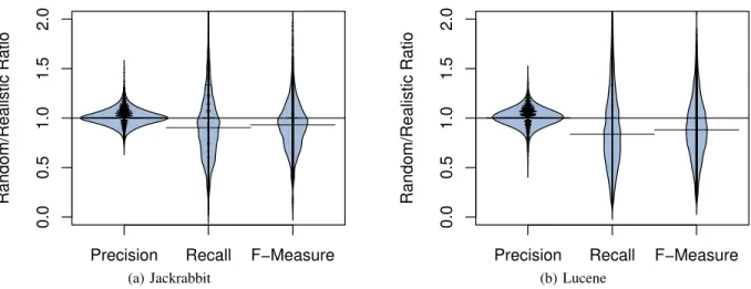
(9) 2.0 1.5 1.0 0.0. 0.5. Realistic/Clean Ratio. 2.0 1.5 1.0 0.5 0.0. Realistic/Clean Ratio. Precision. Recall. F−Measure. (a) Jackrabbit. Precision. Recall. F−Measure. (b) Lucene. Fig. 5: The difference in performance between models trained using realistic noisy samples and clean samples. All models are tested on clean samples (defect mislabelling).. The modules classified as defective by models trained using noisy data are typically as reliable as the modules classified as defective by models trained using clean data. Figure 5 shows that there is a median ratio of one between the precision of models trained using the realistic noisy and clean samples for both of the studied systems. Furthermore, we find that the 95% confidence interval for the distributions are 0.881.20 (Jackrabbit) and 0.90-1.19 (Lucene). This tight range of values that are centred at one suggests that the precision of our models is not typically impacted by mislabelled defects. On the other hand, models trained using noisy data tend to miss more defective modules than models trained using clean data. Figure 5 shows that the median ratio between the recall of models trained using the realistic noisy and clean samples is 0.68 (Jackrabbit) and 0.56 (Lucene). This indicates that models trained using data with mislabelled defects typically achieve 56%-68% of the recall that models trained on clean data would achieve when tested on clean data.. While defect mislabelling rarely impacts the precision of defect models, the recall is often impacted. Practitioners can rely on the modules classified as defective by defect models trained on noisy data. However, cleaning historical data prior to training defect models will likely improve their recall. Random mislabelling issue reports tends to overestimate the impact that realistic mislabelling has on model performance. Figure 6 shows that while the median ratio between the precision of realistic and random noisy models is 1 for both studied systems, the median recall and F-measure ratios are 0.84-0.90 and 0.88-0.93 respectively. In fact, 64%66% of the recall and F-measure ratios are below 1 in our studied systems, indicating that models trained using randomly mislabelled issues tend to overestimate the impact that real mislabelling has on the recall and F-measure of our models.. When randomly injecting mislabelled defects, our results suggest that the impact of the mislabelling will be overestimated by 7-16 percentage points.. (RQ3) How does mislabelling impact the interpretation of defect models? Approach. We again use the high-level approach of Figure 4 to address RQ3. While Step 1 of the approach is identical for RQ2 and RQ3, Steps 2 and 3 are performed differently. We describe the different Steps 2 and 3 below. (Step 2) Analyze models: For each bootstrap iteration, we calculate the variable importance score for each metric in each type of model (i.e., clean, realistic noisy, and random noisy). Hence, the variable importance score for each metric is calculated three times in each bootstrap iteration. (Step 3) Interpret results: We cluster the variable importance scores of metrics in each type of model using Scott-Knott tests to produce statistically distinct ranks of metrics for clean, realistic noisy, and random noisy models. Thus, each metric has a rank for each type of model. To estimate the impact that random and realistic mislabelling have on model interpretation, we compute the difference in the ranks of the metrics that appear in the top-three ranks of the clean models. For example, if a metric m appears in the top rank in the clean and realistic noisy models then the metric would have a rank difference of zero. However, if m appears in the third rank in the random noisy model, then the rank difference of m would be negative two. Similar to RQ2, we repeat the whole experiment for each studied release individually. Results. Figure 7 shows the rank differences for all of the studied releases. We again perform experiments for defect mislabelling and non-defect mislabelling individually. The scarcity of non-defect mislabelling limits the impact that it can have on model interpretation. Indeed, we find that there are very few rank differences in the non-defect mislabelling.

(10) 2.0 1.5 1.0 0.0. 0.5. Random/Realistic Ratio. 2.0 1.5 1.0 0.5 0.0. Random/Realistic Ratio. Precision. Recall. F−Measure. Precision. (a) Jackrabbit. Recall. F−Measure. (b) Lucene. Fig. 6: The difference in performance between models trained using random noisy and realistic noisy samples. All models are tested on clean samples (defect mislabelling).. Realistic Noisy Sample Ranked 1. metrics) do not appear in the second rank of the realistic noisy model, indicating that these metrics are influenced by defect mislabelling. Furthermore, 8%-33% of the second and third rank variables drop by two or more ranks in the noisy models.. Random Noisy Sample. Ranked 2. Ranked 3. 100% 80% Jackrabbit. 60%. Percentage. 40% 20% 0% 100% 80%. Lucene. 60% 40% 20%. The most influential metrics are generally robust to defect mislabelling, with 80%-85% of the most influential metrics from the clean models appearing in the top rank of the noisy models as well. On the other hand, the second and third ranks are unstable, with as little as 18% of the metrics from the clean models appearing in those ranks in the noisy models.. 0% 2. 1. 0 −1 −2 −3 −4 −5. 2. 1. 0 −1 −2 −3 −4 −5. 2. 1. 0 −1 −2 −3 −4 −5. Difference in rank. Fig. 7: The difference in the ranks for the metrics according to their variable importance scores among the clean and noisy models. The bars indicate the percentage of variables that appear in that rank in the clean model while also appearing in that rank in the noisy models.. results. Hence, we focus on defect mislabelling for the remainder of this section. The most influential metrics are generally robust to the noise introduced by defect mislabelling. Figure 7 shows that 80% (Lucene) to 85% (Jackrabbit) of the metrics in the top rank of the clean model (most often, the committer experience) also appear in the top rank of the realistic noisy model. Similarly, 80% (Lucene) to 85% (Jackrabbit) of the metrics in the top rank of the clean model appear in the top rank of the random noisy model. Moreover, the 10%-15% of metrics in the top rank of the clean model that do not appear in the top rank of the noisy models only decrease by one rank. Conversely, the metrics in the second and third ranks are less stable. Figure 7 shows that 31% (Jackrabbit) to 75% (Lucene) of the metrics in the second rank and 38% (Jackrabbit) to 82% (Lucene) of the metrics in the third rank of the clean model (most often, the process and developer. Randomly injected mislabelled defects have a more damaging impact on model interpretation than real mislabelled defects do. Figure 7 shows that a smaller percentage of the metrics of the clean models are found at the same rank in the random noisy models than the realistic noisy models. Randomly injecting mislabelled defects tends to distort the interpretation of influential metrics more than truly mislabelled defects do. V. D ISCUSSION & T HREATS TO VALIDITY We now discuss the results of our case study with respect to other work on issue report mislabelling, as well as the threats to the validity of our case study. A. Discussion In prior work, Herzig et al. show that issue report mislabelling has a drastic impact on the relative order of the most defect-prone files [19] — 16%-40% of the top-10% most defect-prone files do not belong in that group. The impact that issue report mislabelling has on the ordering of the most defect-prone files suggests that defect models (such as the ones that we build in this study) will also be drastically impacted, both in terms of precision and recall..

(11) Yet in this study, we find that issue report mislabelling has little impact on the precision of defect models, which may seem to be incongruent with the prior work. We suspect that the differences in the conclusions that we draw have to do with the differences in our defect prediction experiments. In the study of Herzig et al., files are ranked according to the number of defect reports that are mapped to a file. The files at the top of this ranked list are the most defectprone, and would yield the most benefit from additional quality assurance effort [18]. Instability in the top-10% of files in this ranked list occurs if these highly defect-prone file have several mislabelled defects mapped to them. On the other hand, our defect models classify whether a file is defective or clean. In order for a file to be remapped from defective to clean, all of the defects that are mapped to a file must be mislabelled, reducing the number of defects to zero. Otherwise, a file would still be considered defective. Hence, the instability that Herzig et al. observe with respect to the most defect-prone files may not have as much of an impact on the files that our defect models will consider defective. B. Threats to Validity External validity. We focus our study on two subject systems, due to the low number of systems that satisfied our analysis criteria (cf. Section III). The lack of a curated oracle of mislabelled issue reports presented a major challenge. Nonetheless, additional replication studies are needed. Construct validity. Although the studied datasets have high link rates of issue reports and code changes, we make the implicit assumption that these links are correct. On the other hand, we rely on JIRA links from issue reports to code changes, which others have noted lead to more accurate links than links constructed from code changes to issue reports [40]. Internal validity. We use nine metrics to train models that identify mislabelled issue reports, and ten metrics to train models that identify defective files. We selected metrics that cover a variety of dimensions for each type of model. However, other metrics that we may have overlooked could also improve the performance of our models. We focus on the random forest classification technique. Although prior studies have also used random forest [13, 14, 22, 24, 28], our findings are entirely bound to this technique. We plan to explore the impact that issue report mislabelling has on other classification techniques in future work. VI. C ONCLUSIONS Defect models identify potentially defective software modules. However, the accuracy of the predictions and the insights derived from defect models depend on the quality of the data from which these models are trained. While recent work has shown that issue report mislabelling may impact the performance of defect prediction models [26, 40], the mislabelled issue reports were generated randomly. In this paper, we study the nature of mislabelled issue reports and the impact that truly mislabelled issue reports have on the performance and interpretation of defect models.. Through a case study of two large and successful open source systems, we make the following observations: – Mislabelling is not random. Models trained to identify mislabelled issue reports achieve a mean F-measure that is 4-34 times better than that of random guessing. A reporter’s tendency to mislabel issues in the past is consistently the most influential metric used by our models. – Since we observe that the precision of our defect models is rarely impacted by defect mislabelling, practitioners can rely on the accuracy of modules labelled as defective by defect models that are trained using noisy data — the files that are classified as defect-prone by models trained using noisy data are often just as accurate as the defectprone predictions of models trained using clean data (i.e., mislabel-free). However, cleaning the data prior to training defect models will likely allow them to identify more of the truly defective modules. – The most influential metrics are generally robust to defect mislabelling. 80%-85% of the most influential metrics from the clean models appear in the top ranks of the noisy models as well. – On the other hand, the second- and third-most influential metrics are more unstable than the most influential ones. As little as 18% of the metrics in the second and third influence rank of the clean models also appear in the same rank in the noisy models. – Randomly injecting mislabelled defects tends to overestimate the impact that defect mislabelling has on the performance and interpretation of defect models. ACKNOWLEDGMENTS This work would not have been possible without the manually-curated oracle of mislabelled issue reports provided by Herzig et al. [19]. This work was conducted as a part of the Program for Advancing Strategic International Networks to Accelerate the Circulation of Talented Researchers; and the Japan Society for the Promotion of Science, Grant-in-Aid for Young Scientists (B: 25730045) and Scientific Research (B: 23300009). This work was also supported by the Natural Sciences and Engineering Research Council of Canada (NSERC). R EFERENCES [1] F. Akiyama, “An Example of Software System Debugging,” in Proceedings of the International Federation of Information Processing Societies Congress (IFIP’71), 1971, pp. 353–359. [2] G. Antoniol, K. Ayari, M. D. Penta, and F. Khomh, “Is it a Bug or an Enhancement? A Text-based Approach to Classify Change Requests,” in Proceedings of the IBM Centre for Advanced Studies Conference (CASCON’08), 2008, pp. 1–15. [3] J. Aranda and G. Venolia, “The Secret Life of Bugs: Going Past the Errors and Omissions in Software Repositories,” in Proceedings of the International Conference on Software Engineering (ICSE’09), 2009, pp. 298–308..

(12) [4] E. Arisholm, L. C. Briand, and E. B. Johannessen, “A Systematic and Comprehensive Investigation of Methods to Build and Evaluate Fault Prediction Models,” Journal of Systems and Software, vol. 83, no. 1, pp. 2–17, 2010. [5] A. Bachmann, C. Bird, F. Rahman, P. Devanbu, and A. Bernstein, “The Missing Links: Bugs and Bug-fix Commits,” in Proceedings of the International Symposium on the Foundations of Software Engineering (FSE’10), 2010, pp. 97–106. [6] C. Bird, A. Bachmann, E. Aune, J. Duffy, A. Bernstein, V. Filkov, and P. Devanbu, “Fair and Balanced? Bias in Bug-Fix Datasets,” in Proceedings of the joint meeting of the European Software Engineering Conference and the symposium on the Foundations of Software Engineering (ESEC/FSE’09), 2009, pp. 121–130. [7] C. Bird, B. Murphy, and H. Gall, “Don’t Touch My Code! Examining the Effects of Ownership on Software Quality,” in Proceedings of the joint meeting of the European Software Engineering Conference and the symposium on the Foundations of Software Engineering (ESEC/FSE’11), 2011, pp. 4–14. [8] L. Breiman, “Random Forests,” Machine Learning, vol. 45, no. 1, pp. 5–32, 2001. [9] A. Canty and B. Ripley, boot: Bootstrap R (S-Plus) Functions, 2014. [Online]. Available: http://CRAN. R-project.org/package=boot [10] M. Cataldo, A. Mockus, J. Roberts, and J. Herbsleb, “Software Dependencies, Work Dependencies, and Their Impact on Failures,” Transactions on Software Engineering, vol. 35, no. 6, pp. 864–878, 2009. [11] M. D’Ambros, M. Lanza, and R. Robbes, “An Extensive Comparison of Bug Prediction Approaches,” in Prooceedings of the Working Conference on Mining Software Repositories (MSR’10), 2010, pp. 31–41. [12] R. Efron, B. and Tibshirani, An Introduction to the Bootstrap. Chapman & Hall, 1993. [13] T. Fukushima, Y. Kamei, S. McIntosh, K. Yamashita, and N. Ubayashi, “An Empirical Study of Just-in-Time Defect Prediction using Cross-Project Models,” in Proceedings of the Working Conference on Mining Software Repositories (MSR’14), 2014, pp. 172–181. [14] G. Gousios, M. Pinzger, and A. V. Deursen, “An Exploratory Study of the Pull-Based Software Development Model,” in Proceedings of the International Conference on Software Engineering (ICSE’14), 2014, pp. 345–355. [15] T. Hall, S. Beecham, D. Bowes, D. Gray, and S. Counsell, “A Systematic Literature Review on Fault Prediction Performance in Software Engineering,” Transactions on Software Engineering, vol. 38, no. 6, pp. 1276–1304, 2012. [16] F. E. Harrell Jr., Regression Modeling Strategies, 1st ed. Springer, 2002. [17] A. E. Hassan, “Predicting Faults Using the Complexity of Code Changes,” in Proceedings of the International Conference on Software Engineering (ICSE’09), 2009, pp. 78–88.. [18] A. E. Hassan and R. C. Holt, “The Top Ten List: Dynamic Fault Prediction,” in Proceedings of the International Conference on Software Maintenance (ICSM’05), 2005, pp. 263–272. [19] K. Herzig, S. Just, and A. Zeller, “It’s Not a Bug, It’s a Feature: How Misclassication Impacts Bug Prediction,” in Proceedings of the International Conference on Software Engineering (ICSE’13), 2013, pp. 392–401. [20] K. Herzig and A. Zeller, “The Impact of Tangled Code Changes,” in Proceedings of the Working Conference on Mining Software Repositories (MSR’13), 2013, pp. 121– 130. [21] E. G. Jelihovschi, J. C. Faria, and I. B. Allaman, “ScottKnott: A Package for Performing the Scott-Knott Clustering Algorithm in R,” Tendłncias em Matemtica Aplicada e Computacioal - TEMA., vol. 15, no. 1, pp. 3–17, 2014. [22] Y. Jiang, B. Cukic, and T. Menzies, “Can Data Transformation Help in the Detection of Fault-prone Modules?” in Proceedings of the Workshop on Defects in Large Software Systems (DEFECTS’08), 2008, pp. 16–20. [23] Y. Kamei, E. Shihab, B. Adams, a. E. Hassan, A. Mockus, A. Sinha, and N. Ubayashi, “A Large-Scale Empirical Study of Just-in-Time Quality Assurance,” Transactions on Software Engineering, vol. 39, no. 6, pp. 757–773, 2013. [24] Y. Kamei, S. Matsumoto, A. Monden, K.-i. Matsumoto, B. Adams, and A. E. Hassan, “Revisiting Common Bug Prediction Findings Using Effort-Aware Models,” in Proceedings of the International Conference on Software Maintenance (ICSM’10), 2010, pp. 1–10. [25] P. Kampstra, “Beanplot: A Boxplot Alternative for Visual Comparison of Distributions,” Journal of Statistical Software, vol. 28, no. 1, pp. 1–9, 2008. [26] S. Kim, H. Zhang, R. Wu, and L. Gong, “Dealing with Noise in Defect Prediction,” in Proceeding of the International Conference on Software Engineering (ICSE’11), 2011, pp. 481–490. [27] S. Kim, T. Zimmermann, E. J. Whitehead Jr., and A. Zeller, “Predicting Faults from Cached History,” in Proceedings of the International Conference on Software Engineering (ICSE’07), 2007, pp. 489–498. [28] S. Lessmann, S. Member, B. Baesens, C. Mues, and S. Pietsch, “Benchmarking Classification Models for Software Defect Prediction: A Proposed Framework and Novel Findings,” Transactions on Software Engineering, vol. 34, no. 4, pp. 485–496, 2008. [29] A. Lim, L. Breiman, and A. Cutler, bigrf: Big Random Forests: Classification and Regression Forests for Large Data Sets, 2014. [Online]. Available: http://CRAN.R-project.org/package=bigrf [30] S. McIntosh, Y. Kamei, B. Adams, and A. E. Hassan, “The Impact of Code Review Coverage and Code Review Participation on Software Quality,” in Proceedings of the Working Conference on Mining Software Repositories (MSR’14), 2014, pp. 192–201..

(13) [31] A. Mockus, “Missing Data in Software Engineering,” in Guide to Advanced Empirical Software Engineering, 2008, pp. 185–200. [32] ——, “Organizational Volatility and its Effects on Software Defects,” in Proceedings of the International Symposium on Foundations of Software Engineering (FSE’10), 2010, pp. 117–127. [33] A. Mockus and D. M. Weiss, “Predicting Risk of Software Changes,” Bell Labs Technical Journal, vol. 5, no. 6, pp. 169–180, 2000. [34] R. Moser, W. Pedrycz, and G. Succi, “A Comparative Analysis of the Efficiency of Change Metrics and Static Code Attributes for Defect Prediction,” in Proceedings of the International Conference on Software Engineering (ICSE’08), 2008, pp. 181–190. [35] N. Nagappan, B. Murphy, and V. R. Basili, “The Influence of Organizational Structure on Software Quality: An Empirical Case Study,” in Proceedings of the International Conference on Software Engineering (ICSE’08), 2008, pp. 521–530. [36] N. Nagappan, A. Zeller, T. Zimmermann, K. Herzig, and B. Murphy, “Change Bursts as Defect Predictors,” in Proceedings of the International Symposium on Software Reliability Engineering (ISSRE’10), 2010, pp. 309–318. [37] A. T. Nguyen, T. T. Nguyen, H. A. Nguyen, and T. N. Nguyen, “Multi-layered Approach for Recovering Links between Bug Reports and Fixes,” in Proceedings of the International Symposium on the Foundations of Software Engineering (FSE’12), 2012, pp. 63:1–63:11. [38] T. H. Nguyen, B. Adams, and A. E. Hassan, “A Case Study of Bias in Bug-Fix Datasets,” in Proceedings of the Working Conference on Reverse Engineering (WCRE’10), 2010, pp. 259–268. [39] D. Radjenovic, M. Hericko, R. Torkar, and A. Zivkovic, “Software Fault Prediction Metrics: A Systematic Literature Review,” Information and Software Technology, vol. 55, no. 8, pp. 1397–1418, 2013. [40] F. Rahman and P. Devanbu, “How, and Why, Process Metrics Are Better,” in Proceedings of the International Conference on Software Engineering (ICSE’13), 2013, pp. 432–441. [41] F. Rahman, I. Herraiz, and D. Posnett, “Sample Size vs. Bias in Defect Prediction,” in Proceedings of the joint meeting of the European Software Engineering Conference and the symposium on the Foundations of Software Engineering (FSE’13), 2013, pp. 147–157.. [42] F. Rahman, D. Posnett, A. Hindle, E. Barr, and P. Devanbu, “BugCache for Inspections: Hit or Miss?” in Proceedings of the joint meeting of the European Software Engineering Conference and the symposium on the Foundations of Software Engineering (ESEC/FSE’11), 2011, pp. 322–331. [43] A. J. Scott and M. Knott, “A Cluster Analysis Method for Grouping Means in the Analysis of Variance,” Biometrics, vol. 30, no. 3, pp. 507–512, 1974. [44] C. Seiffert, T. M. Khoshgoftaar, J. Van Hulse, and A. Folleco, “An Empirical Study of the Classification Performance of Learners on Imbalanced and Noisy Software Quality Data,” Information Sciences, vol. 259, pp. 571–595, 2014. [45] E. Shihab, “An Exploration of Challenges Limiting Pragmatic Software Defect Prediction,” Ph.D. dissertation, Queen’s University, 2012. [46] E. Shihab, Z. M. Jiang, W. M. Ibrahim, B. Adams, and A. E. Hassan, “Understanding the Impact of Code and Process Metrics on Post-Release Defects: A Case Study on the Eclipse Project,” in Proceedings of the International Symposium on Empirical Software Engineering and Measurement (ESEM’10), 2010. [47] E. Shihab, Y. Kamei, B. Adams, and A. E. Hassan, “High-Impact Defects: A Study of Breakage and Surprise Defects,” in Proceedings of the joint meeting of the European Software Engineering Conference and the symposium on the Foundations of Software Engineering (ESEC/FSE’11), 2011, pp. 300–310. [48] M. R. Sikonja, “Improving Random Forests,” in Proceedings of the European Conference on Machine Learning (ECML’04), 2004, pp. 359–370. [49] E. J. Weyuker, T. J. Ostrand, and R. M. Bell, “Do too many cooks spoil the broth? Using the number of developers to enhance defect prediction models,” Empirical Software Engineering, vol. 13, no. 5, pp. 539–559, 2008. [50] R. Wu, H. Zhang, S. Kim, and S. C. Cheung, “ReLink: Recovering Links between Bugs and Changes,” in Proceedings of the joint meeting of the European Software Engineering Conference and the symposium on the Foundations of Software Engineering (ESEC/FSE’11), 2011, pp. 15–25. [51] T. Zimmermann, R. Premraj, and A. Zeller, “Predicting Defects for Eclipse,” in Proceedings of the International Workshop on Predictor Models in Software Engineering (PROMISE’07), 2007, pp. 9–20..

(14)