Measurement of Branching Fractions of B→
Xs?+?- Decays at the Belle II experiment
著者
Sato Yo
学位授与機関
Tohoku University
PhD Thesis
Measurement of Branching Fractions of B
→ X
s
!
+
!
−
Decays at
the Belle II experiment
(Belle II
B
→ X
s
!
+
!
−
)
Yo Sato
Department of Physics
Graduate School of Science
Tohoku University
2020
Abstract
The inclusive B ! Xs`+` decays are a great probe to search for physics beyond the standard model
(SM) of particle physics. The process is a flavor-changing-neutral-current (FCNC) process which proceeds via loop diagrams in the standard model and thus are strongly suppressed. Since a new heavy particle might be able to enter the loop, the FCNC is sensitive for new physics. Moreover, B! Xs`+` decays
provide complementary information with less hadronic uncertainty to the exclusive B! K(⇤)`+` decays
in which tensions from the SM prediction have been observed. Belle II is a unique experiment to explore the process with large statistics to shed light on the anomalies.
We performed the measurements of the branching fractions of B ! Xs`+` decay using the data
set accumulated by Belle II experiment which corresponds to 37.7 million BB pairs. This is the first measurement on B! Xs`+` at Belle II experiment. The obtained results are
B(B ! Xse+e ) = [4.86+2.752.42(stat)+1.020.92(syst)]⇥ 10 6 (1)
B(B ! Xsµ+µ ) < 4.67(5.61)⇥ 10 6 at 90%(95%) CL (2)
B(B ! Xs`+` ) < 5.54(6.30)⇥ 10 6 at 90%(95%) CL (3)
Because the statistical significance on B ! Xsµ+µ and B! Xs`+` is less than 2 , the upper limit on
the branching fraction is set for these modes. The branching fraction of B! Xse+e and B! Xsµ+µ
is consistent with previous measurements and the SM prediction. Result of B ! Xs`+` is consistent
with the world average, Belle measurement and the SM prediction, while the di↵erence from BaBar is at 1.4 level.
The analysis procedure of B! Xs`+` decays at Belle II experiment well established and we have
got ready to lead to decisive conclusions regarding the anomalies which are observed in the exclusive B ! K(⇤)`+` decays with upcoming Belle II data.
Acknowledgment
First I am extremely grateful to my supervisors, Prof. Hitoshi Yamamoto and Prof. Tomoyuki Sanuki for their invaluable advice and continuous. It is truly an honor to complete my PhD thesis under their supervision. I also deeply appreciate Prof. Akimasa Ishikawa for his technical support for my study. Without his great support, I could not write my thesis.
I am thankful to all Belle II collaborators, especially the internal referees Prof. Claudia Cecchi, Prof. Gagan Mohanty, and Dr. Racha Cheaib, for many suggestions and advice. I would like to express my gratitude to members of the EWP working group. The EWP conveners Dr. Simon Wehle and Dr. Saurabh Sandilya supported me from the beginning of my study. I also would like to thank members of the Lepton ID performance group for their kind supports for my two-photon study. I would like to o↵er my special thanks to all members of DESY, especially Prof. Carsten Niebuhr, Dr. Samuel Cunli↵e, and Dr. Ilya Komarov, for kind help and support that have made my study and life in Hamburg a wonderful time.
I am deeply grateful to Prof. Enrico Lunghi and Mr. Jack Jenkins for useful discussions and advice from the theoretical aspect. Prof. Enrico Lunghi kindly accepted to be an external examiner for my GP-PU qualifying examination.
I would like to thank late Dr. Tadashi Nagamine and Dr. Ryo Yonamine for their many supports and encouragements. I would like to extend my thanks to the secretary Ms. Kaori Kobayashi for taking care of every official business. I an grateful to spend my PhD course with all members in this laboratory.
My PhD research project was supported JSPS KAKENHI Grant Number JP19J10179 and Graduate Program on Physics for the Universe (GP-PU), Tohoku University.
I would like to thank all my friends who gave me the necessary distraction from my research. Last but not least, I deeply grateful to my family, my father Shigehiko, my mother Yuko, my sister Kinu, my brother Kai and Kai’s wife Hitomi, who gave me invaluable supports and encouraged me.
Sincerely, Yo Sato
Contents
1 Introduction 1 2 Physics Motivation 3 2.1 Overview . . . 3 2.2 E↵ective Hamiltonian . . . 3 2.3 Inclusive B! Xs`+` decays . . . 5 2.4 Exclusive B! K(⇤)`+` decays . . . . 62.5 Constraints on the Wilson coefficients . . . 10
2.6 Interplay of inclusive and exclusive b! s`+` . . . . 10
3 Belle II Experiment 12 3.1 SuperKEKB accelerator . . . 12 3.2 Belle II detector . . . 12 3.2.1 VXD . . . 13 3.2.2 CDC . . . 13 3.2.3 TOP . . . 15 3.2.4 ARICH . . . 17 3.2.5 ECL . . . 20 3.2.6 KLM . . . 21 3.2.7 Trigger . . . 21
3.3 Status of the Belle II experiment . . . 22
3.4 Particle identification (PID) . . . 23
4 Analysis Overview 28 4.1 Analysis strategy . . . 28
4.2 Data sample . . . 28
4.3 Monte-Carlo simulation sample . . . 28
4.3.1 Signal MC sample . . . 29 4.3.2 Background MC sample . . . 29 5 Reconstruction 31 5.1 Particle selection . . . 31 5.2 Xs reconstruction . . . 32 5.3 B reconstruction . . . 32 6 Background Study 35 6.1 Background sources . . . 35 6.2 Background suppression . . . 35 6.2.1 Pre-selection . . . 35 6.2.2 Charmonium veto . . . 36 6.2.3 D veto . . . 39 6.2.4 FastBDT . . . 40
6.2.5 Best candidate selection . . . 44
6.2.6 Summary . . . 44
viii CONTENTS
6.3.1 Double mis-ID background . . . 51
6.3.2 Swapped mis-ID background . . . 53
6.3.3 Charmonium background . . . 53
7 Extraction of the Branching Fraction 55 7.1 Probability density function (PDF) . . . 55
7.1.1 Signal . . . 55 7.1.2 Self cross-feed . . . 56 7.1.3 Non-peaking background . . . 56 7.1.4 Peaking background . . . 57 7.2 Fitter check . . . 59 8 Systematic Uncertainty 61 8.1 Number of B meson pairs . . . 61
8.2 Efficiency correction . . . 61
8.2.1 Charged track reconstruction efficiency . . . 61
8.2.2 Lepton identification efficiency . . . 62
8.2.3 Hadron (K±, ⇡±) identification efficiency . . . . 62
8.2.4 K0 S reconstruction efficiency . . . 62
8.2.5 ⇡0 reconstruction efficiency . . . . 62
8.2.6 FastBDT selection efficiency . . . 62
8.2.7 Summary of the efficiency correction . . . 62
8.3 Fitter bias . . . 62
8.4 PDF uncertainty . . . 63
8.4.1 Uncertainty of signal shape . . . 63
8.4.2 Uncertainty of self cross-feed ratio . . . 63
8.4.3 Uncertainty of peaking background yields . . . 63
8.5 Signal modeling of non-resonant Xs . . . 63
8.5.1 K⇤-X stransition point . . . 64
8.5.2 b-quark mass . . . 64
8.5.3 Fermi motion momentum . . . 64
8.5.4 Fragmentation and missing modes of Xs . . . 65
8.5.5 Fraction of B! K`+` , B ! K⇤`+` , and non-resonant B ! Xs`+` . . . 66
9 Validation with Control Modes 67 9.1 Reconstruction of B! XsJ/ (! `+` ) . . . 67
9.1.1 Signal MC for B+ ! K+⇡ ⇡+J/ . . . . 67
9.2 Branching fraction extraction for B! XsJ/ . . . 69
9.3 Systematic uncertainty for B! XsJ/ . . . 69
9.4 Results on the branching fraction of B! XsJ/ . . . 71
10 Results and Discussion 75 10.1 Results on B! Xse+e and B! Xsµ+µ . . . 75
10.2 Results on B! Xs`+` . . . 77
10.3 Discussion and prospect . . . 77
11 Conclusion 82 A MC Calibration 83 B Lepton ID Efficiency Correction and Uncertainty with Two-photon Events 87 B.1 Introduction . . . 87
B.2 Data set . . . 87
B.3 Data sample . . . 87
B.3.1 Monte-Carlo simulation sample . . . 87
B.4 Selection . . . 87
CONTENTS ix
B.4.2 Trigger selection . . . 88
B.4.3 Tag selection . . . 88
B.5 Lepton ID efficiency calculation . . . 88
B.6 Systematic uncertainty . . . 89
B.6.1 Correction between data and MC . . . 89
B.6.2 Generator e↵ects . . . 89
B.7 Binning definition . . . 90
B.8 Results . . . 90
B.8.1 Electron ID efficiency . . . 90
List of Tables
2.1 Measurements of the branching fraction on B! Xs`+` decays. . . 6
2.2 The SM prediction of the branching fraction on B! Xs`+` decays. . . 6
2.3 Measurements of the branching fraction on B! K(⇤)`+` decays averaged by HFLAV [1]. 8 2.4 The SM prediction of the branching fraction on B! K(⇤)`+` decays. . . . . 8
3.1 Production cross-section and event rate. . . 21
4.1 Decay modes of Xs which are reconstructed in the analysis. . . 28
5.1 Summary of the particle selection criteria. . . 33
6.1 Criteria of the pre-selection . . . 36
6.2 The list of input variables of FastBDT . . . 45
6.3 Classification of samples for FastBDT training and criteria on the output value. . . 51
6.4 Cut flow table of Xse+e . Number of events satisfying each selection, signal efficiency and FOM are shown. Note that the Mbc cut, 5.27 < Mbc < 5.29 GeV/c2 is not imposed. The numbers are scaled for an integrated luminosity of 34.6 fb 1. . . 51
6.5 Cut flow table of Xsµ+µ . Number of events satisfying each selection, signal efficiency and FOM are shown. Note that the Mbc cut, 5.27 < Mbc < 5.29 GeV/c2 is not imposed. The numbers are scaled for an integrated luminosity of 34.6 fb 1. . . 52
7.1 Summary of the probability functions and parameters. . . 55
7.2 Shape parameters of the signal PDF. . . 56
7.3 The ratio of the self cross-feed to the signal estimated by the simulation. . . 56
7.4 Summary of the selection criteria for the B! D⇡ control samples. . . . 57
7.5 Shape parameters of the background PDF. . . 57
7.6 The yields of the peaking backgrounds. . . 59
8.1 The efficiency correction factors on the B! Xs`+` reconstruction. . . 63
8.2 The fragmentation correction factors. . . 66
9.1 Reconstruction efficiency on the control modes B! XsJ/ estimated in MC samples. . 68
9.2 The efficiency correction factors on the B! XsJ/ . . . 69
9.3 Obtained mean and width of the pull distributions on B! XsJ/ control samples. . . . 71
9.4 The branching fractions and corresponding signal yields on B! XsJ/ control samples. 72 9.5 Systematic uncertainties on the branching fraction in unit of 10 4. The total is obtained from the sum in quadrature of all contributions. . . 74
10.1 Central values of the branching fractions and corresponding signal yileds. . . 75
10.2 Systematic uncertainties on the branching fraction in unit of 10 6. The uncertainties are categorized as additive (A) or multiplicative (M). . . 76
10.3 Central value of the branching fractions. . . 77
10.4 Systematic uncertainties on the branching fraction in unit of 10 6. The uncertainties are categorized as additive (A) or multiplicative (M). . . 78
LIST OF TABLES xi
B.1 Summary of the MC samples used in this analysis. . . 88 B.2 Definition of binning for electronID study. . . 90 B.3 Definition of binning for muonID study. . . 91
List of Figures
1.1 Mass reach of the ATLAS searches for SUSY. . . 2
2.1 Feynman diagrams of radiative and electroweak penguin decays in the SM. (a) b! s(d) , (b) b! s(d)`+` , (c) b ! s(d)⌫⌫ . . . 3
2.2 Feynman diagrams of b! s`+` process in the E↵ective Hamiltonian framework. (a) O7 contribution, (b)O9,10 contribution. . . 4
2.3 Measurement of the forward-backward asymmetry in Belle [2]. Black dots with error bars represent the measurement and curve (black) with the band (red) and dashed boxes (black) shows the SM prediction. The backgrounds form J/ (! `+` ) and (2S)( ! `+` ) events have been vetoed by rejected events in the teal hatched regions. For the electron channel, the pink shaded regions are added to the veto regions due to the large bremsstrahlung e↵ect. 7 2.4 Measurement of the CP -averaged observable P50 in LHCb [3]. Black dots with error bars represent the measurement and orange boxes show the SM prediction. . . 9
2.5 Measurement of the lepton-flavor-violating observable Q5 in Belle [4]. Black dots with error bars represent the measurement. Blue boxes show the SM prediction and orange boxed show a prediction in a new-physics model [5] . . . 9
2.6 Measurement of the lepton-flavor-universality test observables RK (Left) and RK⇤ (Right). 10 2.7 Constraints on the Wilson coefficients in (C9NPµ, C NPµ 10 ), (C NPµ 9 , C 0µ 9 ), and (C NPµ 9 , C9NPe) from left to right [6]. NP denotes new-physics contribution, CNP= C CSM. The origin is the SM prediction. The contours of each experiment correspond to the 3 constraint and blue contours of All Data shows 1, 2, 3 constraints. . . 10
2.8 Expected sensitivity on the Wilson coefficients in (CNP 9 , C10NP) from inclusive B! Xs`+` measurements at Belle II [7]. NP denotes new-physics contribution, CNP = C CSM. Black, red and blue lines show 1 , 3 , and 5 level constraints, respectively. Red contours show the current global fits results at level of 1, 2, 3 [8]. . . 11
3.1 Schematic view of the SuperKEKB accelerator. . . 13
3.2 Top view of the Belle II detector. . . 14
3.3 CAD rendering of PXD. . . 14
3.4 Schematic view of SVD longitudinal section. [9] . . . 15
3.5 Wire configuration of Belle CDC (upper) and Belle II CDC (lower). [9] . . . 15
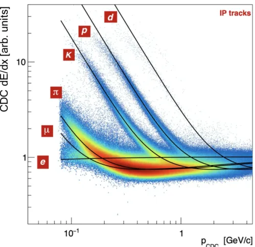
3.6 Energy loss dE/dx at CDC as a function of track momentum. Two dimensional distribu-tions are measured in data and the black solid line shows the predicdistribu-tions with the simulation 16 3.7 Schematic view of a TOP module. [10] . . . 17
3.8 Relation between the hit time and the position of MCP-PMT. Black points shows the data of a kaon. The left side is the pion PDF and the right side is the kaon PDF. [11] . . . 18
3.9 Left : The principle of the particle identification of the ARICH. Right : Principle of operation of the proximity focusing with non-homogeneous aerogel radiator. . . 18
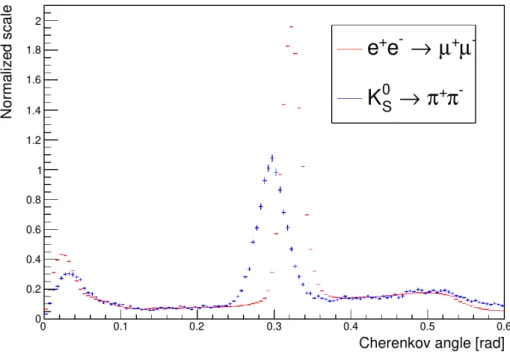
3.10 The Cherenkov angle as a function of track momentum with refractive index n = 1.05. [12] 19 3.11 Distribution of the Cherenkov angle for e+e ! µ+µ sample with muon momentum selection 6.4 GeV/c < p < 7.0 GeV/c in red, and for the K0 S ! ⇡ +⇡ sample with pion momentum selection 1.0 GeV/c < p < 1.1 GeV/c in blue. [13] . . . 19
LIST OF FIGURES xiii
3.12 The E/p distributions for a variety of momentum ranges. Turquoise line is for electron, purple line is for muon and black line is for pion. The peak at 0 means that a track does not much any ECL cluster. [7] . . . 20 3.13 Schematic view of L1 trigger system. CDC find a track using small segment information,
which is called Track Segment Finder (TSF), and reconstruct 2D track. In addition, 3D track information which is constructed from 2D track and beam along information. Neural network based track finder is going to be implemented. ECL provides both each cluster information and total energy deposit in ECL to GRL. TOP and KLM information helps to identify particle type at the trigger level. . . 22 3.14 Luminosity integration in Phase 3 until 2020 summer. . . 23 3.15 P ID distributions. (a) P IDe, (b) P IDµ, (c) P ID⇡, (d) P IDK. Red line shows electron,
orange line shows muon, blue line shows pion, and green line shows kaon. . . 24 3.16 Lepton identification efficiency and mis-ID rate from hadron to lepton. Top: Electron
identification at P IDe> 0.9, Bottom: Muon identification at P IDµ> 0.9. Note that the
mis-ID rate has been inflated by a factor 3 for illustration purposes. [14] . . . 26 3.17 Hadron identification performance as a function ofRK/⇡. Kaon identification efficiency is
shown with triangle and mis-ID rate from pion to kaon is inverted triangle. Red is data and blue is MC. [15] . . . 27
4.1 MXs distribution for generated signal MC samples. The histograms are scaled to the 200
fb 1. Decay modes of Xs are separated by color code of histogram. . . 30
5.1 MK0 S distribution of K 0 S ! ⇡ +⇡ in the MC samples. . . . 32 5.2 M distribution of ⇡0 ! in the MC samples. . . 32 5.3 MXs distribution of signal MC samples. . . 33
5.4 Mbc (left) and E (right) distributions of the signal MC samples. Green line is B !
Xse+e and blue line is B! Xsµ+µ . . . 34
6.1 E distributions of B ! Xs`+` . Red line shows the signal events, blue line shows
background events from BB events, and green line shows background events from qq continuum events. . . 36 6.2 MXs distributions of B ! Xs`
+` . Red line shows the signal events, blue line shows
background events from BB events, and green line shows background events from qq continuum events. . . 37 6.3 Me+e distributions of B ! Xse+e . Red line shows the signal events, blue line shows
background events from BB events, and green line shows background events from qq continuum events. The qq continuum background has a peak at Me+e = 0 due to photon
conversion and Dalitz decay of ⇡0. . . . 37
6.4 Me+( )e ( ) and Mµ+µ distributions. Red line shows the signal events, blue line shows
background events from BB events, and green line shows background events from qq continuum events. The BB background has peaks at M`+` = 3.0969 GeV/c2 due to J/
and at M`+` = 3.6861 GeV/c2due to (2S). . . 38
6.5 MmostD likedistributions of events which are identified as the double mis-ID background
using the MC truth information. Decay modes of Xs are separated by color. The
his-tograms are scaled for an integrated luminosity of 34.6 fb 1. . . 39 6.6 Mbcdistributions before applying the FastBDT. MC samples are identified by color code.
White histogram shows signal events. The histograms are scaled for an integrated lumi-nosity of 34.6 fb 1. . . 40 6.7 Schematic view of the application of FastBDT. The depth of trees is three in this case. . . 41 6.8 Top : E distributions of B ! Xse+e with fitting functions. Black makers with error
bar show the distribution of MC samples. Red line shows the total likelihood distribution and blue and cyan lines show each component of Crystal Ball function. Bottom : Pull (=[data - fit]/[statistical uncertainty]) distribution of E. . . 44
xiv LIST OF FIGURES
6.9 Top : E distributions of B! Xsµ+µ with fitting functions. Black makers with error
bar show the distribution of MC samples. Red line shows the total likelihood distribution and blue and cyan lines show each component of Crystal Ball function. Bottom : Pull
(=[data - fit]/[statistical uncertainty]) distribution of E. . . 45
6.10 FastBDT input variables of B! Xse+e (1) KSFW variables. Red line shows the signal events, blue line shows background events from BB events, and green line shows back-ground events from qq continuum events. . . 46
6.11 FastBDT input variables of B ! Xse+e (2) CLEO Cone variables and other variables. Red line shows the signal events, blue line shows background events from BB events, and green line shows background events from qq continuum events. . . 47
6.12 FastBDT input variables of B ! Xsµ+µ (1) KSFW variables. Red line shows the signal events, blue line shows background events from BB events, and green line shows background events from qq continuum events. . . 48
6.13 FastBDT input variables of B! Xsµ+µ (2) CLEO Cone variables and other variables. Red line shows the signal events, blue line shows background events from BB events, and green line shows background events from qq continuum events. . . 49
6.14 FastBDT output distributions. Red line shows the signal events, blue line shows back-ground events from BB events, and green line shows backback-ground events from qq continuum events. . . 50
6.15 Mbc distributions after the background suppression. The colors indicate di↵erent MC samples. White histogram shows signal events. The histograms are scaled for an integrated luminosity of 34.6 fb 1. . . 52
6.16 Estimated Mbc distributions of the double mis-ID backgrounds. MC samples are identified by color code. Red line shows total peaking component and blue shows non-peaking component. The histograms are scaled for an integrated luminosity of 34.6 fb 1. . . 53
6.17 Estimated Mbc distributions of the swapped mis-ID backgrounds. MC samples are identi-fied by color code. Red line shows total peaking component and blue shows non-peaking component. The histograms are scaled for an integrated luminosity of 34.6 fb 1. . . 54
6.18 Estimated Mbc distributions of the Charmonium backgrounds. The histograms are scaled for an integrated luminosity of 34.6 fb 1. . . 54
7.1 Mbc distributions of the B ! XsJ/ control samples in data. The fit contained the following components: a Gaussian for the signal (red line) and an ARGUS function to model background from the continuum and combinatorial B decays (dashed blue line). . . 56
7.2 Mbc PDF of the self cross-feed. . . 57
7.3 Mbc distributions of the B ! D⇡ control samples in data. The fit contained the follow-ing components: a Gaussian for the signal (red line) and an ARGUS function to model background from the continuum and combinatorial B decays (dashed blue line). . . 58
7.4 Mbc PDF of the double mis-ID background. . . 58
7.5 Mbc PDF of the swapped mis-ID background. . . 58
7.6 Mbc PDF of the Charmonium background. . . 59
7.7 Pull distributions of signal yields. . . 60
8.1 MXs distributions for various b-quark mass. Black line shows the distribution of mb = 4.80 GeV/c2, red line shows that of m b = 4.65 GeV/c2, and blue line shows that of mb = 4.95 GeV/c2. . . . 64
8.2 M`+` distributions for various b-quark mass. Black line shows the distribution of mb = 4.80 GeV/c2, red line shows that of m b = 4.65 GeV/c2, and blue line shows that of mb = 4.95 GeV/c2. . . . 64
8.3 MXs distributions for various Fermi motion momentum. Black dashed line shows the distribution of pF = 0.410 GeV, black line shows the distribution of pF = 0.461 GeV, red line shows the distribution of pF = 0.422 GeV, and blue line shows the distribution of pF = 0.498 GeV. . . 65
LIST OF FIGURES xv
8.4 M`+` distributions for various Fermi motion momentum. Black dashed line shows the
distribution of pF = 0.410 GeV, black line shows the distribution of pF = 0.461 GeV, red
line shows the distribution of pF = 0.422 GeV, and blue line shows the distribution of
pF = 0.498 GeV. . . 65
9.1 MK+⇡ ⇡+ distribution at the MC truth level which is used to estimated the reconstruction efficiency. Black line shows the total distribution. Contributions from each process is identified by color code. . . 68
9.2 Pull of number of signal distributions of the B! XsJ/ (! e+e ). . . 70
9.3 Pull of number of signal distributions of the B! XsJ/ (! µ+µ ). . . 70
9.4 Mbc distributions of the B ! XsJ/ (! e+e ) with fitting function. The fit contained the following components: a Gaussian for the signal (red line) and an ARGUS function to model background from the continuum and combinatorial B decays (dashed blue line). The total fit is the solid blue line and the data are overlaid as black makers. . . 71
9.5 Mbc distributions of the B ! XsJ/ (! µ+µ ) with fitting function. The fit contained the following components: a Gaussian for the signal (red line) and an ARGUS function to model background from the continuum and combinatorial B decays (dashed blue line). The total fit is the solid blue line and the data are overlaid as black makers. . . 72
9.6 Measurements results on the branching fractions of B! XsJ/ modes. Black dots show the world average, blue dots show the our results with electron modes, and green dots show the our results with muon modes. The internal error bars show only the statistical uncertainty and outer ones show the uncertainty combined statistical and systematic one. 73 10.1 Mbc distributions of the B ! Xs`+` with the fitting function. The fit contained the following components: a Gaussian for the signal (red line), an ARGUS function to model background from the continuum and combinatorial B decays (dashed blue line), a his-togram PDF to describe self cross-feed (dashed green line), and three hishis-togram PDFs to describe peaking backgrounds, (i) double mis-ID background (dashed light-blue line), (ii) swapped mis-ID background (dashed magenta line), (iii) Charmonium background (dashed orange line). The total fit result is the solid blue line and the data are overlaid as black makers. . . 75
10.2 Mbcdistributions of the B! Xs`+` with the fitting function when the simultaneous fit-ting is applied. The fit contained the following components: a Gaussian for the signal (red line), an ARGUS function to model background from the continuum and combinatorial B decays (dashed blue line), a histogram PDF to describe self cross-feed (dashed green line), and three histogram PDFs to describe peaking backgrounds, (i) double mis-ID back-ground (dashed light-blue line), (ii) swapped mis-ID backback-ground (dashed magenta line), (iii) Charmonium background (dashed orange line). The total fit is the solid blue line and the data are overlaid as black makers. . . 77
10.3 Negative log-likelihood statistical-only profiles for the branching fraction of B! Xs`+` . 79 10.4 Measurement results of the branching fractions of B! Xs`+` . Red lines show results of this analysis, green lines show BaBar measurements [16], blue lines show Belle measure-ment [17], and black lines show the world average [1]. The internal error bars show only the statistical uncertainty and outer ones show the uncertainty combined statistical and systematic one. Yellow band show the SM prediction 2.2. . . 80
A.1 E distributions of B! K+`+` with the fitting function . . . . 84
A.2 E distributions of B! K+⇡0`+` with the fitting function . . . . 85
A.3 Mean of the Crystal Ball function and its di↵erence between data and MC . . . 85
A.4 Width of the Crystal Ball function and its di↵erence between data and MC . . . 86
B.1 Momentum of the probe particle and M`+` distributions after the electron ID probe selection. Black line shows the data sample and red line shows background events estimated with MC. MC distributions are multiplied by 10 for visualization purpose. . . 89
B.2 Momentum of the probe particle and M`+` distributions after the muon ID probe selec-tion. Black line shows the data sample and red line shows background events estimated with MC. MC distributions are multiplied by 10 for visualization purpose. . . 90
xvi LIST OF FIGURES
B.3 Electron ID efficiency of data for P IDe> 0.9. . . 91
B.4 Ratio of electron ID efficiency between data and MC for P IDe> 0.9. . . 92
B.5 Electron ID efficiency of data for P IDµ> 0.9. . . 93
Chapter 1
Introduction
The Standard Model (SM) of elementary particle physics is an outstanding theory to match various experiment results. The SM consists of quark and lepton which compose matter, gauge interaction, and the Higgs mechanism. Higgs boson which was the last piece of SM has been discovered in ATLAS and CMS experiment in 2012 [18] [19]. Despite great successes, the SM is thought to be not perfect theory. There remain some open questions, for example, absence of the dark matter candidates, and a description of gravity is not included in the SM. Therefore, the e↵ort to search for physics beyond the SM from both experimental and theoretical aspects is highly motivated.
Experiment with high energy accelerator is a promising tool for new physics exploration. There are two kinds of experiments in this field, energy frontier experiment and intensity frontier one. In the energy frontier experiment, a direct production of new particles is main target process. Some new physics models such as supersymmetry (SUSY) [20, 21, 22, 23, 24, 25] predict new heavy particles. The highest centre-of-mass energy is around 13 TeV by LHC (Large Hadron Collider) and mass reach at ATLAS and CMS experiments for new heavy particle isO(1) TeV. Figure 1.1 shows the mass reach for SUSY at ATLAS. Currently, no evidence of new particles is observed, which may suggest new physics candidates exist higher thanO(1) TeV.
While, the intensity frontier experiments perform precise measurements with high statistics data to probe new physics. One of the most promising processes in the intensity frontier experiments is the flavor-changing-neutral-current (FCNC) process, such as a b! s`+` transition. The FCNC is suppressed in
the SM and proceeds mainly via loop diagrams. New heavy particles might be able to enter the loops or even proceed the FCNC process at tree diagram level, which leads deviations on observables from the SM prediction.
In the analysis of B ! K(⇤)`+` decays, which is proceeded by b
! s`+` at the quark level,
some tensions with the SM have been reported by LHCb [3] [26] [27], Belle [4], and ATLAS [28]. The deviation from the SM in an angular observable, so-called P0
5, in B ! K⇤µ+µ decays is at 2.9 level
[3]. In the measurement of the ratio of branching fraction between muon modes and electron modes RK(⇤) = B(B ! K(⇤)µ+µ )/B(B ! K(⇤)µ+µ ), the deviation at 2.5 level has been observed [26]
[27]. The mass scale of new physics behind the anomalies is O(10) TeV which is much higher than the centre-of-mass energy of Belle and BaBar. Furthermore, these measurement may imply a violation of the lepton flavor universality (LFU). In the SM, three charged leptons e, µ and ⌧ are identical except for the Yukawa couplings and thus masses. The LFU violation is a clear evidence of physics beyond the SM and may provide a hint for the fermion generation problem.
Inclusive B ! Xs`+` decays provide a complementary information to exclusive B ! K(⇤)`+` .
The hadronic uncertainties in inclusive decays are under better control and are largely independent of those in exclusive ones. All existing B ! Xs`+` measurements are highly statistically limited due to
the limited data sample. The Belle II experiment, which is a successor of Belle, is a unique experiment to perform measurements on inclusive B ! Xs`+` decays. Sensitivity at Belle II with full integrated
luminosity is expected to be sufficient to play a decisive role to search for new physics.
In this paper, we report the measurement of the branching fractions of B! Xs`+` decays at Belle
II experiment. We use a data sample containing 37.7⇥ 106 BB pairs corrected by Belle II with the
SuperKEKB accelerator. This is the first measurement on B! Xs`+` decays at Belle II and opens a
2
Model Signature RL dt [fb1] Mass limit Reference
In cl us iv e S ea rc he s 3 rdgen. squar ks di rect pr oduct ion EW direc t Long-liv ed par tic les RP V ˜q˜q, ˜q!q˜0 1 0 e, µ 2-6 jets ETmiss 139 m( ˜0 1)<400 GeV ATLAS-CONF-2019-040 1.9 ˜q [10⇥ Degen.]
mono-jet 1-3 jets Emiss
T 36.1 m(˜q)-m( ˜0 1)=5 GeV 1711.03301 0.71 ˜q [1⇥, 8⇥ Degen.] 0.43 ˜q [1⇥, 8⇥ Degen.] ˜g˜g, ˜g!q¯q˜0 1 0 e, µ 2-6 jets ETmiss 139 m( ˜0 1)=0 GeV ATLAS-CONF-2019-040 2.35 ˜g m( ˜0 1)=1000 GeV ATLAS-CONF-2019-040 1.15-1.95 ˜g ˜g Forbidden ˜g˜g, ˜g!q¯qW ˜0 1 1 e, µ 2-6 jets 139 m( ˜0 1)<600 GeV ATLAS-CONF-2020-047 2.2 ˜g ˜g˜g, ˜g!q¯q(``) ˜0
1 ee, µµ 2 jets ETmiss 36.1 m(˜g)-m( ˜0
1)=50 GeV 1805.11381 1.2 ˜g ˜g˜g, ˜g!qqWZ ˜0 1 0 e, µ 7-11 jets ETmiss 139 m( ˜0 1) <600 GeV ATLAS-CONF-2020-002 1.97 ˜g SS e, µ 6 jets 139 m(˜g)-m( ˜0 1)=200 GeV 1909.08457 1.15 ˜g ˜g˜g, ˜g!t¯t˜0 1 0-1 e, µ 3 b ETmiss 79.8 m( ˜0 1)<200 GeV ATLAS-CONF-2018-041 2.25 ˜g SS e, µ 6 jets 139 m(˜g)-m( ˜0 1)=300 GeV 1909.08457 1.25 ˜g ˜b1˜b1, ˜b1!b ˜0 1/t ˜± 1 Multiple 36.1 m( ˜0 1)=300 GeV, BR(b ˜0 1)=1 1708.09266, 1711.03301 0.9 ˜b1 ˜b1 Forbidden Multiple 139 m( ˜0 1)=200 GeV, m( ˜± 1)=300 GeV, BR(t ˜± 1)=1 1909.08457 0.74 ˜b1 ˜b1 Forbidden ˜b1˜b1, ˜b1!b ˜0 2! bh ˜0 1 0 e, µ 6 b ETmiss 139 m( ˜0 2, ˜01)=130 GeV, m( ˜0 1)=100 GeV 1908.03122 0.23-1.35 ˜b1 ˜b1 Forbidden 2 ⌧ 2 b Emiss T 139 m( ˜0 2, ˜0 1)=130 GeV, m( ˜0 1)=0 GeV ATLAS-CONF-2020-031 0.13-0.85 ˜b1 ˜b1 ˜t1˜t1, ˜t1!t ˜0 1 0-1 e, µ 1 jet ETmiss 139 m( ˜0 1)=1 GeV ATLAS-CONF-2020-003, 2004.14060 1.25 ˜t1 ˜t1˜t1, ˜t1!Wb ˜0 1 1 e, µ 3 jets/1 b ETmiss 139 m( ˜0 1)=400 GeV ATLAS-CONF-2019-017 0.44-0.59 ˜t1
˜t1˜t1, ˜t1!˜⌧1b⌫, ˜⌧1!⌧ ˜G 1 ⌧ + 1 e,µ,⌧ 2 jets/1 b Emiss
T 36.1 ˜t1 1.16 m(˜⌧1)=800 GeV 1803.10178 ˜t1˜t1, ˜t1!c ˜01/˜c˜c, ˜c!c˜01 0 e, µ 2 c ETmiss 36.1 m( ˜0 1)=0 GeV 1805.01649 0.85 ˜c m(˜t1,˜c)-m( ˜0 1)=50 GeV 1805.01649 0.46 ˜t1 0 e, µ mono-jet Emiss T 36.1 m(˜t1,˜c)-m( ˜0 1)=5 GeV 1711.03301 0.43 ˜t1 ˜t1˜t1, ˜t1!t ˜0 2, ˜0 2!Z/h ˜0 1 1-2 e, µ 1-4 b Emiss T 139 m( ˜0 2)=500 GeV SUSY-2018-09 0.067-1.18 ˜t1 ˜t2˜t2, ˜t2!˜t1+Z 3 e, µ 1 b Emiss T 139 m( ˜0 1)=360 GeV, m(˜t1)-m( ˜0 1)=40 GeV SUSY-2018-09 0.86 ˜t2 ˜t2 Forbidden ˜± 1˜02via WZ 3 e, µ Emiss T 139 m( ˜0 1)=0 ATLAS-CONF-2020-015 0.64 ˜± 1/ ˜02
ee, µµ 1 jet Emiss
T 139 m( ˜± 1)-m( ˜0 1)=5 GeV 1911.12606 0.205 ˜± 1/ ˜02 ˜± 1˜⌥1via WW 2 e, µ Emiss T 139 m( ˜0 1)=0 1908.08215 0.42 ˜± 1 ˜± 1˜02via Wh 0-1 e, µ 2 b/2 Emiss T 139 m( ˜0 1)=70 GeV 2004.10894, 1909.09226 0.74 ˜± 1/ ˜0 2 ˜± 1/ ˜0 2 Forbidden ˜± 1˜⌥1via ˜`L/˜⌫ 2 e, µ ETmiss 139 m(˜`,˜⌫)=0.5(m( ˜± 1)+m( ˜0 1)) 1908.08215 1.0 ˜± 1 ˜⌧˜⌧, ˜⌧!⌧˜0 1 2 ⌧ ETmiss 139 m( ˜0 1)=0 1911.06660 0.12-0.39 ˜⌧ [˜⌧L, ˜⌧R,L] 0.16-0.3 ˜⌧ [˜⌧L, ˜⌧R,L] ˜`L,R˜`L,R, ˜`!` ˜0 1 2 e, µ 0 jets ETmiss 139 m( ˜0 1)=0 1908.08215 0.7 ˜`
ee, µµ 1 jet Emiss
T 139 m(˜`)-m( ˜0 1)=10 GeV 1911.12606 0.256 ˜` ˜ H ˜H, ˜H!h ˜G/Z ˜G 0 e, µ 3 b Emiss T 36.1 BR( ˜0 1! h ˜G)=1 1806.04030 0.29-0.88 ˜H 0.13-0.23 ˜H 4 e, µ 0 jets Emiss T 139 BR( ˜0 1! Z ˜G)=1 ATLAS-CONF-2020-040 0.55 ˜H Direct ˜+ 1˜1prod., long-lived ˜±
1 Disapp. trk 1 jet ETmiss 36.1 ˜± 0.46 Pure Wino 1712.02118
1
Pure higgsino ATL-PHYS-PUB-2017-019
0.15
˜± 1
Stable˜g R-hadron Multiple 36.1 ˜g 2.0 1902.01636,1808.04095
Metastable˜g R-hadron, ˜g!qq˜0 1 Multiple 36.1 m( ˜0 1)=100 GeV 1710.04901,1808.04095 2.4 ˜g [⌧( ˜g) =10 ns, 0.2 ns] 2.05 ˜g [⌧( ˜g) =10 ns, 0.2 ns] ˜± 1˜⌥1/ ˜01, ˜±
1!Z`!``` 3 e, µ 139 ˜⌥ 1.05 Pure Wino ATLAS-CONF-2020-009
1/ ˜01 [BR(Z⌧)=1, BR(Ze)=1] 0.625 ˜⌥ 1/ ˜01 [BR(Z⌧)=1, BR(Ze)=1] LFV pp!˜⌫⌧+X, ˜⌫⌧!eµ/e⌧/µ⌧ eµ,e⌧,µ⌧ 3.2 0 311=0.11,132/133/233=0.07 1607.08079 1.9 ˜⌫⌧ ˜± 1˜⌥1/ ˜02! WW/Z````⌫⌫ 4 e, µ 0 jets Emiss T 36.1 m( ˜0 1)=100 GeV 1804.03602 1.33 ˜± 1/ ˜0 2 [i33, 0,12k, 0] 0.82 ˜± 1/ ˜0 2 [i33, 0,12k, 0] ˜g˜g, ˜g!qq˜0 1, ˜0
1! qqq 4-5 large-R jets 36.1 Large00
112 1804.03568 1.9 ˜g [m( ˜0 1)=200 GeV, 1100 GeV] 1.3 ˜g [m( ˜0 1)=200 GeV, 1100 GeV] Multiple 36.1 m( ˜0
1)=200 GeV, bino-like ATLAS-CONF-2018-003
2.0 ˜g [00 112=2e-4, 2e-5] 1.05 ˜g [00 112=2e-4, 2e-5] ˜t˜t, ˜t!t ˜0 1, ˜0 1! tbs Multiple 36.1 m( ˜0
1)=200 GeV, bino-like ATLAS-CONF-2018-003
1.05 ˜t [00 323=2e-4, 1e-2] 0.55 ˜t [00 323=2e-4, 1e-2] ˜t˜t, ˜t!b˜± 1, ˜± 1! bbs 4b 139 m( ˜± 1)=500 GeV ATLAS-CONF-2020-016 0.95 ˜t ˜t Forbidden ˜t1˜t1, ˜t1!bs 2 jets + 2 b 36.7 ˜t˜t11[qq, bs][qq, bs] 0.42 0.61 1710.07171 ˜t1˜t1, ˜t1!q` 2 e, µ 2 b 36.1 ˜t1 0.4-1.45 BR(˜t1!be/bµ)>20% 1710.05544 1 µ DV 136 ˜t1 [1e-10<0 1.6 BR(˜t1!qµ)=100%, cos✓t=1 2003.11956
23k<1e-8, 3e-10<023k<3e-9] 1.0
˜t1 [1e-10<0
23k<1e-8, 3e-10<023k<3e-9]
Mass scale [TeV]
101 1
ATLAS SUSY Searches* - 95% CL Lower Limits
July 2020 ATLAS Preliminaryps = 13 TeV
*Only a selection of the available mass limits on new states or phenomena is shown. Many of the limits are based on simplified models, c.f. refs. for the assumptions made.
FIG 1.1: Mass reach of the ATLAS searches for SUSY.
The outline of this thesis is as follows. The physics motivation of this thesis and measurements on b! s`+` are described in Chapter 2. The Belle II experiment and SuperKEKB accelerator are explained in
Chapter 3. An overview on the analysis procedure is given in Chapter 4. Event reconstruction procedure is described in Chapter 5. Methods of background suppression and peaking background estimation are described in Chapter 6. A method of the branching fraction extraction is explained in Chapter 7. Sources of systematic uncertainty are listed and estimation methods are decried in Chapter 8. Measurement of the branching fraction on B ! XsJ/ control samples is shown for validation of the analysis procedure
in Chapter 9. Obtained results of the branching fraction of B ! Xs`+` and discussion are described in
Chapter 2
Physics Motivation
2.1
Overview
The goal of this thesis is to perform the measurement of the branching fraction of B ! Xs`+` decays
as the first measurement on the B! Xs`+` process at the Belle II experiment.
Radiative penguin b! s(d) decay and electroweak penguin b ! s(d)`+` and b
! s(d)⌫⌫ decays are FCNC processes. Thanks to the presence of photons and leptons in the final state, the size of non-perturbative QCD corrections can be reduced compared with fully hadronic decay. Figure 2.1 shows the SM Feynman diagrams of these decays. In the SM, t-quark and weak bosons Z0, W± which are much
heavier than b-quark mediate the process. New heavy particles may enter the loop or even proceed via tree diagrams, which induce a deviation on observables with the SM prediction. Thus, these processes are a good probe to search new physics.
The B! K`+` decay has been firstly observed by Belle in b
! s`+` transition [29]. The branching
fraction of b ! s`+` is O(10 6) which is two orders of magnitude smaller than b ! s because of
additional vertex leading ↵emfactor. On the other hand, due to the two leptons, an angular analysis can
provide rich information to explore new physics. In this chapter, we introduce the theoretical framework and measurements on b! s`+` . ! "/$ % & ' (a) b! s(d) ! "/$ % ! "/$ % & & & '/( ℓ ℓ ℓ ℓ (b) b! s(d)`+` ! "/$ % ! "/$ % & & & ' ) ℓ ) ) ) (c) b! s(d)⌫⌫
FIG 2.1: Feynman diagrams of radiative and electroweak penguin decays in the SM. (a) b! s(d) , (b) b! s(d)`+` , (c) b
! s(d)⌫⌫
2.2
E↵ective Hamiltonian
Flavor changing process is described from wide mass scale from ⇤QCD ⇠ 400 MeV over mb ⇠ 4.3 GeV
to MW = 80.4 GeV and Mt ⇠ 165 GeV. In scale of mb and above, the QCD e↵ects can be calculated
with perturbation theory, though it is difficulty for the dynamics associated with the energy scale ⇤QCD.
The e↵ective Hamiltonian is described using the operator product expansion technique to separate these di↵erent scales [30] [31] [32]. In this framework, the e↵ective Hamiltonian for b ! s transitions in the SM are given by [33] HSMe↵ = 4GF p 2 " s t 10 X i=1 Ci(µ)Oi(µ) + su 2 X i=1 Ci(µ)(Oi(µ) Oiu(µ)) # (2.1)
where GF is the Fermi constant, sqis a product of CKM matrix elements such as st= VtbVts⇤, and µ is the
energy scale at which the calculation is being performed. There is the unitary relation, s
4 2.2. EFFECTIVE HAMILTONIAN
0. The Oi are local operators providing the “long-distance” descriptions. The each operator has an
associated Wilson coefficient Ci which describes “short-distance” physics with the perturbation theory.
The Wilson coefficients Ci are evaluated at a scale µW which is of the order of the W -boson mass. The
renormalization group equation can be used to evolve the Ci to the scale µb which is of the order of the
mb.
Expressions of the current-current (O1,2), photonic dipole (O7), gluonic dipole (O8), and the vector
and axial-vector of electroweak penguin (O9 andO10) are described as follows:
O1= (sL µTacL)(cL µTabL), (2.2) O2= (sL µcL)(cL µbL), (2.3) O7= e 16⇡2mb(sL µ⌫b R)Fµ⌫, (2.4) O8= e 16⇡2mb(sL µ⌫Tab R)Gaµ⌫, (2.5) O9= e 16⇡2mb(sL µbL) X ` (` µ`), (2.6) O10= e 16⇡2mb(sL µbL) X ` (` µ 5`). (2.7)
where Taare the SU(3)
c generators, Fµ⌫ and Gaµ⌫ are the photon and gluon field-strength tensors. The
subscripts L and R represent the chirality of the quark fields. The operatorsOu
1,2are obtained fromO1,2
by replacing the c-quark by u-quark fields. The sums run over the quark flavors q = u, d, s, c, b. The same set of operators for b! d processes can be written by replacing s-quark and d-quark fields. The values of the Wilson coefficient C1,2⇠ 1 at the µb scale. In comparison, C3,4,5,6 are very small at the scale and
hence contributions from the four-quark (O3,4,5,6) operators
O3= (sL µbL) X q (q µq), (2.8) O4= (sL µTabL) X q (q µTaq), (2.9) O5= (sL µ1 µ2 µ3bL) X q (q µ1 µ2 µ3q), (2.10) O6= (sL µ1 µ2 µ3T ab L) X q (q µ1 µ2 µ3Taq). (2.11)
can be neglected. In the electroweak penguin decays b ! s`+` , the operators
O7,9,10 are the most
relevant. Figure 2.2 shows the Feynman diagrams of b ! s`+` process in the E↵ective Hamiltonian
framework. The values of Wilson coefficients are followings, C7(µb) = 0.330, C9(µb) = 4.069, C10(µb) =
4.231 [34] [35]. The e↵ects of new physics beyond the SM can appear through modified values of Wilson coefficients and/or through additional operators with di↵erent chirality or flavor structure.
!
"
ℓ
ℓ
$
!
!
(a)O7 contribution!
"
ℓ
ℓ
$
!,#$
(b)O9,10 contributionFIG 2.2: Feynman diagrams of b ! s`+` process in the E↵ective Hamiltonian framework. (a)
O7
CHAPTER 2. PHYSICS MOTIVATION 5
2.3
Inclusive B
! X
s`
+` decays
Inclusive B ! Xs`+` decays, where Xs is an inclusive hadronic state including a s-quark, provide
information to the b ! s`+` process with good theoretical predictions. Compared with exclusive
B ! K(⇤)`+` decays, the hadronic uncertainty is under better control. Complementary information to
the exclusive decays can be provided to shed light on the anomalies.
There are two main kinematic variables in B! Xs`+` , the di-lepton invariant mass-squared q2 =
M`+` and the angle between direction of `+ [` ] and initial direction of B0 or B [B0or B+] in the
di-lepton centre-of-mass system ✓`. Two observables have been discussed in inclusive B ! Xs`+` decays,
the q2 spectrum d /dq2 [36] and the forward-backward asymmetry dA
F B/dq2 [37]. They are mainly
related to C7, C9and C10 and can be derived at lowest order as followings,
d dq2 = 0m 3 b(1 s)2 (|C9|2+|C10|2)(1 + 2s) + 4 s|C7| 2(2 + s) + 12Re(C⇤ 7C9) , (2.12) dAF B dq2 = Z 1 1 dz d 2 dq2dzsign(z) = 3 0m 3 b(1 s)2sRe ✓ C10 ✓ C9+2 sC7 ◆◆ . (2.13) where s = q2/m2 b, z = cos ✓` and 0= G2 F 48⇡3 ↵2 em 16⇡2|VtbV ⇤ ts|2. (2.14)
An agular decomposition provides a third observable which has di↵erent dependency to the Wilson coefficients. The double-di↵erential decay width can be written as following [38].
d2 dq2d cos ✓ ` = 3 8[(1 + cos 2✓ `)HT(q2) + 2 cos ✓`HA(q2) + 2(1 cos2✓`)HL(q2)] (2.15)
The q2 spectrum and the forward-backward asymmetry can be derived from the functions H i(q2), d dq2 = HT(q 2) + H L(q2), (2.16) dAF B dq2 = 3 4HA(q 2). (2.17)
The functions Hi(q2) are
HT(q2) = 0m3b· 2s(1 s)2 (|C9+ 2 sC7| 2+ |C10|2 , (2.18) HL(q2) = 0m3b· (1 s)2 ⇥ (|C9+ 2C7|2+|C10|2⇤, (2.19) HA(q2) = 9 4 0m 3 b(1 s)2sRe ✓ C10 ✓ C9+ 2 sC7 ◆◆ . (2.20)
Additional information on the Wilson coefficients can be obtained from the lepton flavor universality test observables, RXs[q 2 0, q12] = Rq2 1 q2 0 dq 2 d (B!Xsµ+µ ) dq2 Rq2 1 q2 0 dq 2 d (B!Xse+e ) dq2 . (2.21)
Prediction of RXs in the SM is unity with high precision due to the lepton flavor universality. Taking
interference BSM e↵ect with the SM into account, RXs can be approximated by [39]
RXs' 1 + ( ++ )/2, (2.22) ±= 2 |CSM 9 |2+|C10SM|2 2 4 X i=9,10 Re⇣CiSM(C NPµ i + C 0µ i ) ⌘ + X i=9,10 Re⇣CiSM(CiNPe+ C 0e i ) ⌘3 5 (2.23) C0 is the Wilson coefficient of the chirality flipped operator which is zero in the SM. The labels SM and NP denote the SM and new-physics contributions, respectively (CNP= C CSM).
6 2.4. EXCLUSIVE B! K(⇤)`+` DECAYS
Measurements of B
! X
s`
+`
Belle and BaBar experiments have already performed measurements on B ! Xs`+` [40] [17] [2] [41]
[16]. So far, all measurements are highly statistically limited due to the small branching fraction and limited data sample.
The branching fraction has been measured in Belle using 152⇥ 106 BB pairs [17] and in BaBar
using 471⇥ 106 BB pairs [16]. The measurements and world average by Heavy Flavor Averaging Group
(HFLAV) [1] is summarized in TABLE 2.1. The SM prediction on the branching fraction is shown in TABLE 2.2 [42] [35]. All measurements are consistent with the SM predictions. While measurement of RXs has not been performed in previous experiments, the measurements of the branching fraction at
BaBar correspond to RXs = 0.57
+0.18
0.17 assuming the systematic uncertainties are negligible in the RXs
due to taking ratio. The di↵erence from the unity is at 2.4 level. This is also consistent with the trend of RK(⇤)anomalies which are discussed in the following section. Belle II will perform measurements using
large statistics leading smaller statistical uncertainty.
TABLE 2.1: Measurements of the branching fraction on B! Xs`+` decays.
Experiment B(B ! Xse+e ) [10 6] B(B ! Xsµ+µ ) [10 6] B(B ! Xs`+` ) [10 6] Belle (M`+` > 0.2 GeV) 4.05± 1.30+0.870.83 4.13± 1.05+0.850.81 4.11± 0.83+0.850.81 BaBar (M2 `+` > 0.1 GeV 2) 7.69+0.82+0.71 0.77 0.60 4.41 +1.31+0.63 1.17 0.50 6.73 +0.70+0.60 0.64 0.56
World Average (HFLAV) 6.67± 0.82 4.27+0.980.91 5.84± 0.69
TABLE 2.2: The SM prediction of the branching fraction on B! Xs`+` decays.
B(B ! Xse+e ) [10 6] B(B ! Xsµ+µ ) [10 6] B(B ! Xs`+` ) [10 6]
6.89± 1.01
4.2± 0.7 (M`+` > 0.2 GeV) 4.15± 0.70 4.18± 0.70
The forward-backward asymmetry is firstly measured in Belle using 772⇥ 106 BB pairs [2] as a
function of q2. Figure 2.3 shows the measurement of the forward-backward asymmetry and the SM
prediction. The measurement is consistent with the SM prediction.
To shed further light on the anomalies which are observed in exclusive modes, precise study on inclusive B! Xs`+` is important. The B! Xs`+` decays are reconstructed with a sum-of-exclusive
method, in which Xsis reconstructed from a lot of exclusive final states. High reconstruction efficiency for
stable particles are essential for multiplicity final states. The B-factory experiment at a electron-positron collider is suitable for the analysis on B! Xs`+` thanks to the low background environment. Belle II
is a unique experiment to achieve the measurements on B! Xs`+` with large statistics. Thanks to the
large statistics, angular decomposition measurement, which has not performed due to small statistics, will be performed in Belle II.
Also a fully-inclusive reconstruction method of B ! Xs`+` decays, which has been used in B !
Xs decays, is being explored with dedicated simulation studies. Only di-lepton `+` is reconstructed
explicitly and Xsstate is obtained as the recoil in this method. Efficient background suppression is key
to the success.
2.4
Exclusive B
! K
(⇤)`
+` decays
In the exclusive B! K(⇤)`+` decays, q2 and ✓
` are also important kinematic observables. In addition
to them, two helicity angles ✓K and can be used in B! K⇤(! K⇡)`+` decays. The ✓K is the angle
between the direction of K [K] and that of B [B] in the rest frame of K⇤[K⇤] and is the angle between
CHAPTER 2. PHYSICS MOTIVATION 7
]
2
/c
2
[GeV
2
q
0
5
10
15
20
FB
A
-1.0
-0.5
0.0
0.5
1.0
FIG 2.3: Measurement of the forward-backward asymmetry in Belle [2]. Black dots with error bars represent the measurement and curve (black) with the band (red) and dashed boxes (black) shows the SM prediction. The backgrounds form J/ (! `+` ) and (2S)(
! `+` ) events have been vetoed by
rejected events in the teal hatched regions. For the electron channel, the pink shaded regions are added to the veto regions due to the large bremsstrahlung e↵ect.
Following the definition given in [43], the CP -averaged angular distribution can be written
1 d( + /dq2) d4( + ) dq2d cos ✓ `d cos ✓Kd = 9 32⇡ 3 4(1 FL) sin 2✓ K+ FLcos2✓K +1 4(1 FL) sin 2✓ Kcos 2✓`
FLcos2✓Kcos 2✓`+ S3sin2✓Ksin2✓`cos 2
+ S4sin 2✓Ksin 2✓`cos + S5sin 2✓Ksin ✓`cos
+4
3AF Bsin
2✓
Kcos ✓`+ S7sin2✓Ksin ✓`sin
+ S8sin 2✓Ksin 2✓`sin + S9sin2✓Ksin2✓`sin 2 ⇤. (2.24)
where FL is the fraction of the longitudinal polarication of the K⇤ meson and Si are CP -averaged
observables [43]. To cancel the B! K⇤ form-factor uncertainties, other notation of observables are also
defined. P4,5,6,80 = S4,5,6,8 p FL(1 FL) . (2.25)
Each observable has independent dependence to the Wilson coefficient and can be compared with the SM prediction. The exclusive B ! K⇤`+` provides rich information to set constraints on the Wilson
coefficients from these observables.
In analogy to RXs, the lepton flavor universality observables RK(⇤) have additional information to the
Wilson coefficient. RK(⇤)[q20, q12] = Rq21 q2 0 dq 2 d (B!K(⇤)µ+µ ) dq2 Rq2 1 q2 0 dq 2 d (B!K(⇤)e+e ) dq2 . (2.26)
8 2.4. EXCLUSIVE B! K(⇤)`+` DECAYS
Even though they are also estimated to be equal to unity in the SM, they have other chirality dependency due to the polarization. In lowest order, they can be written using ± 2.23
RK ' 1 + +, (2.27)
RK⇤ ' 1 + + p( + ). (2.28)
where p' 0.86 is the so-called polarization fraction of the K⇤. To solve the chirality structures of lepton
flavor universality violating new-physics, the correlation of RK, RK⇤ and RXs is important. Furthermore,
the double ratios of these variables provide theoretically clean information [39].
Measurements of B
! K
(⇤)`
+`
Exclusive B ! K(⇤)`+` decays are reconstructed from long-lived particles which can be directly
recon-structed and intermediate particles such as K⇤, K0
S, ⇡
0 which are formed from the stable particles. The
B-factory experiments, Belle and BaBar, have advantages on the reconstruction efficiency on electron modes thanks to the high resolution electromagnetic calorimeter. Also the neutral particle such as , ⇡0
and K0
S can be detected efficiently. Experiments with hadron collier, such as LHCb, CMS, ATLAS, and
CDF have large statistics of B meson and high muon reconstruction efficiency, and thus an advantage on the muon modes.
The branching fraction of B ! K(⇤)`+` has been measured in BaBar [44] [45] and Belle [46].
The CDF experiment has also performed measurement on B ! K(⇤)µ+µ [47]. The world average by
HFLAV [1] on the branching fraction of B ! K(⇤)`+` is shown in TABLE 2.3. TABLE 2.4 shows the
SM prediction on the branching fraction [42] [35]. The uncertainties on the predictions are large compared with those of B ! Xs`+` shown in TABLE 2.2 due to the irreducible form factor uncertainty.
TABLE 2.3: Measurements of the branching fraction on B! K(⇤)`+` decays averaged by HFLAV [1].
Mode e+e [10 6] µ+µ [10 6] `+` [10 6]
B! K`+` 0.44
± 0.06 0.44± 0.04 0.48± 0.04 B! K⇤`+` 1.19+0.17
0.16 1.06± 0.09 1.05± 0.10
TABLE 2.4: The SM prediction of the branching fraction on B ! K(⇤)`+` decays.
Mode e+e [10 6] µ+µ [10 6]
B ! K`+` 0.35
± 0.12 0.35± 0.12 B ! K⇤`+` 1.58± 0.49 1.19± 0.39
In the angular measurements and the lepton flavor universality tests, anomalies have been observed on the decays by many experiments. As shown in FIG 2.4, LHCb experiment has reported a discrepancy in the P50 variables with B0 ! K⇤0µ+µ decay at 2.5 and 2.9 level in the 4.0 < q2 < 6.0 GeV
2
and 6.0 < q2< 8.0 GeV2 regions, respectively [3]. Belle experiment has performed the angular analysis using
B ! K⇤e+e and B
! K⇤µ+µ separatly [4]. In the observable P0
5, a tension by 2.6 in q22 [4, 8] GeV2
is observed in the muon mode. In the same region, the electron mode deviates by 1.3 . Measurement of the lepton-flavor-violating observables Q5= P
0µ
5 P
0e
5 has been performed in Belle for the first time.
Figure 2.5 shows the measurement Q5 which is compared with the SM prediction and a new-physics
model given in [5].
LHCb measurements of RK = 0.846+0.060+0.0160.054 0.014in q22 [1.1, 6.0] GeV
2[26] and R
K⇤ = 0.69+0.110.07±0.05
in q2
2 [1.1, 6.0] GeV2[27] deviates by 2.5 and 2.5 from the unity. Measurement on BaBar [45] and Belle [46] are compatible with the SM prediction and the LHCb results. Figure 2.6 summarizes measurements on RK and RK⇤.
CHAPTER 2. PHYSICS MOTIVATION 9
0
5
10
15
]
4
c
/
2
[GeV
2
q
1
−
0.5
−
0
0.5
1
5
'
P
(1S)
ψ/
J
(2S)
ψ
LHCb Run 1 + 2016
SM from DHMV
FIG 2.4: Measurement of the CP -averaged observable P50 in LHCb [3]. Black dots with error bars
represent the measurement and orange boxes show the SM prediction.
6
TABLE I. Fit results for P
4and P
5for all decay channels and separately for the electron and muon modes. The first uncertainties
are statistical and the second systematic.
q2 in GeV2/c2 P40 P4e0 P4µ0 P50 P5e0 P5µ0 [1.00, 6.00] 0.45+0.230.22± 0.09 0.72+0.400.39± 0.06 0.22+0.350.34± 0.15 0.23+0.210.22± 0.07 0.22+0.390.41± 0.03 0.43+0.260.28± 0.10 [0.10, 4.00] 0.11+0.320.31± 0.05 0.34+0.410.45± 0.11 0.38+0.500.48± 0.12 0.47+0.270.28± 0.05 0.51+0.390.46± 0.09 0.42+0.390.39± 0.14 [4.00, 8.00] 0.34+0.180.17± 0.05 0.52+0.240.22± 0.03 0.07+0.320.31± 0.07 0.30+0.190.19± 0.09 0.52+0.280.26± 0.03 0.03+0.310.30± 0.09 [10.09, 12.90] 0.18+0.280.27± 0.06 - 0.40+0.330.29± 0.09 0.17+0.250.25± 0.01 - 0.09+0.290.29± 0.02 [14.18, 19.00] 0.14+0.260.26± 0.05 0.15+0.410.40± 0.04 0.10+0.390.39± 0.07 0.51+0.240.22± 0.01 0.91+0.360.30± 0.03 0.13+0.390.35± 0.06
FIG. 3. Q
4and Q
5observables with SM and favored NP
“Scenario 1” from Ref. [
9
].
by 2.5 (including systematic uncertainty). All
measure-ments are compatible between lepton flavors. The Q
4,5observables are presented in Table
II
and Fig.
3
, where
no significant deviation from zero is discerned.
In conclusion, the first lepton-flavor-dependent angular
analysis measuring the observables P
40and P
50in the B
!
K
⇤`
+`
decay is reported and the observables Q
4,5are
shown for the first time. The results are compatible with
SM predictions, where the largest discrepancy is 2.6 in
P
50for the muon channels.
TABLE II. Results for the lepton-flavor-universality-violating
observables Q
4and Q
5. The first uncertainty is statistical and
the second systematic.
q2 in GeV2/c2 Q4 Q5
[1.00, 6.00] 0.498± 0.527 ± 0.166 0.656± 0.485 ± 0.103 [0.10, 4.00] 0.723± 0.676 ± 0.163 0.097± 0.601 ± 0.164 [4.00, 8.00] 0.448± 0.392 ± 0.076 0.498± 0.410 ± 0.095 [14.18, 19.00] 0.041± 0.565 ± 0.082 0.778± 0.502 ± 0.065
We thank the KEKB group for excellent operation
of the accelerator; the KEK cryogenics group for
effi-cient solenoid operations; and the KEK computer group,
the NII, and PNNL/EMSL for valuable computing and
SINET4 network support.
We acknowledge support
from MEXT, JSPS, and Nagoyas TLPRC (Japan); ARC
(Australia); FWF (Austria); NSFC (China); MSMT
(Czechia); CZF, DFG, and VS (Germany); DST (India);
INFN (Italy); MOE, MSIP, NRF, GSDC of KISTI, and
BK21Plus (Korea); MNiSW and NCN (Poland); MES
and RFAAE (Russia); ARRS (Slovenia); IKERBASQUE
and UPV/EHU (Spain); SNSF (Switzerland); NSC and
MOE (Taiwan); and DOE and NSF (USA).
[1] R. Aaij et al. (LHCb Collaboration),
JHEP 02, 104
(2016)
,
arXiv:1512.04442 [hep-ex]
.
[2] R. Aaij et al. (LHCb Collaboration),
JHEP 09, 179
(2015)
,
arXiv:1506.08777 [hep-ex]
.
[3] R. Aaij et al. (LHCb Collaboration),
Phys. Rev. Lett.
113, 151601 (2014)
,
arXiv:1406.6482 [hep-ex]
.
[4] S. Descotes-Genon, L. Hofer, J. Matias, and J. Virto,
JHEP 06, 092 (2016)
,
arXiv:1510.04239 [hep-ph]
.
[5] W. Altmannshofer and D. M. Straub,
Eur. Phys. J. C75,
382 (2015)
,
arXiv:1411.3161 [hep-ph]
.
[6] W. Altmannshofer, P. Ball, A. Bharucha, A. J. Buras,
D. M. Straub,
and M. Wick,
JHEP 01, 019 (2009)
,
arXiv:0811.1214 [hep-ph]
.
[7] S. Descotes-Genon, J. Matias, M. Ramon, and J. Virto,
JHEP 01, 048 (2013)
,
arXiv:1207.2753 [hep-ph]
.
[8] S. Descotes-Genon, T. Hurth, J. Matias, and J. Virto,
JHEP 05, 137 (2013)
,
arXiv:1303.5794 [hep-ph]
.
[9] B. Capdevila, S. Descotes-Genon, J. Matias,
and
J. Virto,
JHEP 10, 075 (2016)
,
arXiv:1605.03156
[hep-ph]
.
[10] A. Abashian et al. (Belle Collaboration), Nucl. Instrum.
FIG 2.5: Measurement of the lepton-flavor-violating observable Q5 in Belle [4]. Black dots with error
bars represent the measurement. Blue boxes show the SM prediction and orange boxed show a prediction in a new-physics model [5]
10 2.5. CONSTRAINTS ON THE WILSON COEFFICIENTS
Supplementary material to LHCb-PAPER-2019-009
] 4 c / 2 [GeV 2 q 0 5 10 15 20 K R 0.0 0.5 1.0 1.5 2.0 BaBar Belle LHCb Run 1 LHCb Run 1 + 2015 + 2016
LHCb
Figure 1: Comparison of the LHCb RKmeasurements with previous experimental results from
LHCb [1] and the B factories [2, 3]. The LHCb Run 1 result is greyed out since it is superseded by the new result.
Figure 2: Fits to the m (2S)(K+`+` ) invariant-mass distribution of (left)
B+! (2S)(! e+e )K+ and (right) B+! (2S)(! µ+µ )K+ candidates. Electron
(muon) candidates are required to have 9.92 < q2< 16.40 GeV2/c4(12.5 < q2< 14.2 GeV2/c4).
1 0 5 10 15 20 q2 [GeV2/c4] 0.0 0.5 1.0 1.5 2.0 RK ⇤ 0 LHCb LHCb BaBar Belle
FIG 2.6: Measurement of the lepton-flavor-universality test observables RK (Left) and RK⇤ (Right).
2.5
Constraints on the Wilson coefficients
A model-independent global fit based on the E↵ective Hamiltonian framework is powerful way to search for new physics. In addition to the measurements which are discussed in previous sections, other mea-surements on Bs ! µ+µ [48] [49] [50] and Bs ! µ+µ [51] are combined to set constraints on the
Wilson coefficients. Constraints on the Wilson coefficients are investigated by several groups [6] [52]. Figure 2.7 shows contours in 2D planes of the Wilson coefficients given by [6]. The di↵erence between the SM prediction and best fit values is at more than 5 level for these three cases. Smaller C9 than the SM
prediction only in the muon mode is favored from the fits, which may imply the lepton flavor universality
violation. 4
FIG. 1. From left to right: Allowed regions in the (CNP
9µ,C10µNP), (C9µNP,C90µ) and (C9µNP,C9eNP) planes for the corresponding 2D
hypotheses, using all available data (fit “All”) upper row or LFUV fit lower row.
FIG. 2. Preferred regions (at the 1, 2 and 3 level) for the Lµ L model of Ref. [17] from b! s`+` data (green) in the
(mQ, mD) plane with YD,Q= 1. The contour lines denote the predicted values for R[1.1,6]K (red, dashed) and R[1.1,6]K⇤ (blue,
solid).
FIG 2.7: Constraints on the Wilson coefficients in (C9NPµ, C NPµ 10 ), (C NPµ 9 , C 0µ 9 ), and (C NPµ 9 , C9NPe) from
left to right [6]. NP denotes new-physics contribution, CNP= C CSM. The origin is the SM prediction.
The contours of each experiment correspond to the 3 constraint and blue contours of All Data shows 1, 2, 3 constraints.
2.6
Interplay of inclusive and exclusive b
! s`
+`
An impact from the Belle II measurements on inclusive B! Xs`+` decays with an integrated luminosity
of 50 ab 1 to the anomalies which have been observed on exclusive B ! K(⇤)`+` is discussed in this
section. The sensitivities for inclusive B! Xs`+` observables are estimated in [7]. From the branching
fraction and forward-backward asymmetry, the constraints on the Wilson coefficients C9 and C10 are
derived. Contours shown in FIG 2.8 are the Belle II sensitivities for each significance. For example, CNP
CHAPTER 2. PHYSICS MOTIVATION 11
Figure 2.8 also shows red contours which are global fit results mainly from analyses on exclusive decays [8]. If the true values are at the global fit result, the inclusive analyses will exclude the SM with 6 level. Moreover, the hadronic uncertainty of inclusive transition is independent with that of exclusive decay. Thus, a cross-check of analyses on exclusive decays can be performed. Inclusive B ! Xs`+`
measurements at Belle II play a critical role to search for new physics.
1 2 3 4 5 6 77 88 10 10
Belle-2 Projections: Inclusive b sll
Huber, Ishikawa, Virto '2016
Contours: SM Pull with50/ab: BR & AFB
Red: Exclusive Fit (arXiv:1510.04239 [hep-ph])
-2.0 -1.5 -1.0 -0.5 0.0
0.5
1.0
1.5
-1.0
-0.5
0.0
0.5
1.0
1.5
2.0
C
9NPC
10 NPFig. 92: Exclusion contours in the C
9
NP
– C
10
NP
plane resulting from future inclusive b
! s`
+
`
measurements at Belle II. For comparison the constraints on C
9
NP
and C
10
NP
following from
the global fit presented in [595] is also shown.
The B
! K
(
⇤)
⌫ ¯
⌫ decays provide clean testing grounds for new dynamics modifying the
b
! s transition [596–598]. Unlike in other B-meson decays, factorisation of hadronic and
leptonic currents is exact in the case of B
! K
(
⇤)
⌫ ¯
⌫ because the neutrinos are electrically
neutral. Given the small perturbative and parametric uncertainties, measurements of the
B
! K
(
⇤)
⌫ ¯
⌫ decay rates would hence in principle allow to extract the B
! K
(
⇤)
form factors
to high accuracy.
Closely related to the B
! K
(
⇤)
⌫ ¯
⌫ modes are the B decays that lead to an exotic final
state X, since the missing energy signature is the same. Studies of such signals are very
interesting in the dark matter context and may allow to illuminate the structure of the
couplings between the dark and SM sectors [599].
B
! K
(
⇤)
⌫ ¯
⌫ in the SM.
Due to the exact factorisation, the precision of the SM prediction
for the branching ratios of B
! K
(
⇤)
⌫ ¯
⌫ is mainly limited by the B
! K
(
⇤)
form factors
and by the knowledge of the relevant CKM elements. The relevant Wilson coefficient is
known in the SM, including NLO QCD and NLO EW correction to a precision of better
than 2% [387, 388, 390]. Concerning the form factors, combined fits using results from LCSRs
at low q
2
and lattice QCD at high q
2
can improve the theoretical predictions.
Using
(s)
t
= (4.06
± 0.16) · 10
2
for the relevant CKM elements, obtained using unitarity
and an average of inclusive and exclusive tree-level determinations of
|V
cb
|, as well as a
combined fit to LCSR [404] and lattice QCD [600] results for the B
! K
⇤
form factors, one
obtains the following SM prediction for the B
! K
⇤
⌫ ¯
⌫ branching ratio [601]
Br(B
! K
⇤
⌫ ¯
⌫)
SM
= (9.6
± 0.9) · 10
6
.
(271)
248/690
FIG 2.8: Expected sensitivity on the Wilson coefficients in (C9NP, C10NP) from inclusive B ! Xs`+`
measurements at Belle II [7]. NP denotes new-physics contribution, CNP = C CSM. Black, red and
blue lines show 1 , 3 , and 5 level constraints, respectively. Red contours show the current global fits results at level of 1, 2, 3 [8].


![FIG. 2: K-efficiencies and ⇡-mis-ID rates are calculated for different PID criteria using the decay D ⇤+ ! D 0 [K ⇡ + ]⇡ + .](https://thumb-ap.123doks.com/thumbv2/123deta/5889044.1047722/45.892.187.692.392.797/fig-efficiencies-rates-calculated-different-criteria-using-decay.webp)


