Dynamics of the fluid balancer (Diversity and Universality of Nonlinear Wave Phenomena)

Dynamics

of

the fluid balancer

Mikael

A. Langthjem

\dagger,

Tomomichi

Nakamura\ddagger

\dagger Faeulty

_of

Engineering, Yamagata University, Jonan4-chome, Yonezawa, 992-8510Japan

\ddagger Department

_of

Mechanical Engineering,

Osaka

Sangyo University, S-l-l NoJcagaito, Daito-shi, Osaka,

_574-85S001

Japan

Abstract

Thepaperis$\alpha\ovalbox{\tt\small REJECT}$utth the dynamios

of

aso-called

fluu

balatecer;ahulahoop

–g-like smdun containing a small arnount

_of

liquid which, durin rotation, is span out to $fmn$ athin liquid layer on the iner

surface

of

the ring. The liquidis able to $mMemd$ $wMnoe$massin anelastically mounted rotor. The paper derives the equations

_of

motion

for

$d\kappa$coupled

fluid-structure

system, suith the

fluid

equationsbasedonshallowwatertheory.

An analytical aoledion to asinplified version

_of

the shdlow waterequatio , describing a

hydraulic jump, is discussedindetail.

1

Introduction

A fluidbalancerisused

on

rotatingmachinerytoeliminate theundaeirable$eff\infty ts$ofunbalance

mass.

It hasbmme

a

standard feature

on

most household washing machines,but is alsoused

on

heavyindustnial rotating machinery. Tbhngthe washing machine fluid balanoer

as

example, it $\infty nsists$of

a

hollowning, like

a

hulahoop ringbut typioellywith $r\infty\tan g_{J}1ar$

cross

sections,

which cont$\dot{u}$

ns

a

smallamountof liquid. When the ring is rotating at

a

high angular velocity$\Omega$

theliquidwillfom athinliquidlayer

on

the innersurfaceof theoutemostwall,

as

sketchedin

Fig. 1. Consider the situation where

an

unbalanoe

mass

$m$ is present; for example the clothes

inawashingmachine. The rotor hasacriticalangular velocity$\Omega_{cr}$ wherethecentripetalforoes

are

in balancewith the forces due to the restoringspmgs. Below this velocity $(\Omega<\Omega_{er})$ the

mass

centerofthe fluid will belocated ‘onthe

same

side’

as

the unbalance mass,

_as

shownin the left partof Fig. 1. [Here $M$indicatesthe

mass

of the emptyrotor and $\mathcal{M}$ the

mass

of the

$\infty$ntaind liquid.] At acertain supercritical angular velocity $(\Omega>\Omega_{er})$ the

mass

centerofthe

liquidwill

move

tothe’oppositeside’ of the unbalance mass,asshown in the right partof Fig.

1, resultingin ‘massbalance’ andthusinareduoedoedlation amplitude of the rotor.

Figure 1: Workingprincipleofthefluid balancer.

This is the working principleof the fluidbalanoer, which has been verified$\ovalbox{\tt\small REJECT}$tally

[1]; but

no

$\infty ndtl\dot{a}ve$explanation has beengiven

so

far. It is theaim of thepresent projectto

Thepresentworkbuilds upon alargenumber ofstudies into the dynamicsand stabihtyof rotors partiaUyfilled withliquid [2, 3]. Non-linear studies havebeen camiedout by Beman $et$

al. [4], Coldmg-Jorgensen [5], Kasahara etal. [6], and Yoshizumi [7]. Beman et al. [4] found,

both by numerical analysis and by experiment, that non-linear surfaces

can

exist in the fom

ofhydraulic jumps, umdular bores, and solitary

waves.

[An undular bore is arelatively weak

hydraulic jump, with undulations behind it.] Coldin$g$-Jorgensen [5] studiedsolely

a

hydraulic

jump solution, inthespirit ofthe analysis of [4]. Onthe contraryto [4] and [5] the studiesof

Kasahara etal. [6] and Yoshizumi [7]

are

purelynumerical.

To the best of

our

knowledge, theeffect of

an

unbalance

mass

has not been studiedbefore.

The system (with

an

unbalance mss) is however closely related to the so-called automatic

dynamicbalancer [8] where

a

number ofballsrunning inacirculargrooveplaythe

sam

role

as

the liquid layer in the presentstudy.

As

[5] the present study is based largely

on

the approach ofBeman et al. [4]. However,

$\infty ntrary$ to the one-degree-of-freedom assumptionin [4, 5], the presentwork$\infty$nideoe a rotor

withtwodegreesoffreedom.

2

Rotor equation

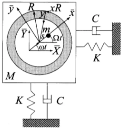
Consider arotatingvessel (rotatingfluidchamber) of

mass

$M$equippedwithasmallunbalance

mass

$m$located adistance $s$fromthegeometric center,and_{$\infty nt-ng$}

a

small amountofliquid,

as

sketchedin Fig. 2. The innerradius of the vessel is $R$

.

Therotoris supported by springs,

with spring constant $K$, in the $\overline{X}$

and $\overline{Y}$

directions. The structural dmpioe forces in these directions are proportional to the parameter $C$

.

Let the $\infty$oidinate system $(\overline{x},\overline{y})$ rotate with

the constantangular velocity$\Omega$ about the fixedsystem (X,Y).

Figure2: Definitionofcoordinatesystemsand

some

ofthe symbolsused. In temsofthe fixed$\infty$ordinatesystemtheequationof motion of the rotor isgivenby

$\{\begin{array}{ll}M+m 00 M+m\end{array}\}\{\begin{array}{l}.\cdot X_{r}.\cdotY_{r}\end{array}\}+\{\begin{array}{ll}C 00 C\end{array}\}\{\begin{array}{l}\dot{X}_{r}\dot{Y}_{r}\end{array}\}$ (1)

$+$ $\{\begin{array}{ll}K_{x} 00 K_{y}\end{array}\}\{\begin{array}{l}X_{r}Y_{r}\end{array}\}=ms\Omega^{2}\{\begin{array}{l}\infty s\Omega ts\dot{m}\Omega t\end{array}\}+\{\begin{array}{l}F_{X}F_{Y}\end{array}\}$

.

Here$X_{r}$and$Y_{r}$

are

thedeflections of the rotor and$F_{Y},$ $F_{Y}$

are

thefluid force$\infty mponents$acting

thereon. An ‘overdot’ denotes differentiation withrespectto time$t$

.

The first tem

on

the right

hand side shows that, in a fixed coordinate system, the unbalance

mss

introduces aperiodic

lt will, however, be

more

$\infty nvenient$ to consider the $\infty upld$fluid-rotor motionin tmsof

therotating$\infty ordinate$system $(\overline{x},\overline{y})$

.

The deflaetionsinthetwo

coordinate

systms

are

related

bythe transfomations

$\{\begin{array}{l}x_{r}y_{r}\end{array}\}=\{\begin{array}{ll}m\Omega t s\dot{m}\Omega t-s\dot{m}\Omega t c\oe\Omega t\end{array}\}\{\begin{array}{l}X_{r}Y_{r}\end{array}\}$ , $\{\begin{array}{l}X_{r}Y_{\prime}\end{array}\}=\{\begin{array}{ll}\infty s\Omega t -s\dot{m}\Omega ts\dot{m}\Omega t c\infty\Omega t\end{array}\}\{\begin{array}{l}x_{r}y_{r}\end{array}\}$

.

(2)

Applying (2) to (1)

we

obtaintheequation of motion intermsofrotating$\infty ordinat\alpha$

as

$\{\begin{array}{ll}M+m 00 M+m\end{array}\}\{\begin{array}{l}.\cdot x_{r}\ddot{y}_{r}\end{array}\}+\{\begin{array}{ll}C -2(M+m)\Omega 2(M+m)\Omega C\end{array}\}\{\begin{array}{l}\dot{x}_{r}\dot{y}_{\prime}\end{array}\}$

$+$ $\{K_{x} -(M+m)\Omega^{2}C\Omega -C\Omega K_{y}-(M+m)\Omega^{2}\}\{\begin{array}{l}x_{r}y_{r}\end{array}\}$ (S)

$=$ $\{\begin{array}{l}ms\Omega^{2}0\end{array}\}+\{\begin{array}{l}F_{x}F_{y}\end{array}\}$

.

It is

seen

that, in this coordinate system, the unbalancemassintroduces

a

foroe, proportional

to $\Omega^{2}$

, actingin thex-direction.

In order to evaluatethekdy foroe $\infty ting$

on

the fluid, the meleration vectorexpressed in

the rotating coordinate systm will beneeded;ltisgivenby

$\{\begin{array}{l}.\cdot X_{r}.\cdot\mathfrak{Y}_{r}\end{array}\}=\{\begin{array}{ll}1 00 l\end{array}\}\{\begin{array}{l}\mathfrak{X}_{r}\ddot{y}_{r}\end{array}\}+2\Omega\{\begin{array}{l}0-l10\end{array}\}\{\begin{array}{l}\dot{x}_{\prime}\dot{y}_{r}\end{array}\}-\Omega^{2}\{\begin{array}{ll}l 00 1\end{array}\}\{\begin{array}{l}x_{r}y_{r}\end{array}\}$

.

(4)

3

Fluid equations

3.1 The

shaUow

water equations

The fluidmotion in the rotatin$g_{V\infty}1$will be described by

a

shalow water approximationof

the Navier-Stokesequations, and intermsof

a

$\infty$ordinatesystem $(x,y)$ attached to thewall of

therotor,

as

shown in Fig. 2. This coordinate system isrelated to

a

polar$\infty ordInate$ system

$(r,\theta)$ attached to the rotor (suchthat$\overline{x}=rcoe\theta,\overline{y}=r$sin$\theta$) inthe foUowing way

$x=R\theta$, $y=R-r$, (5)

where $R$is the radius of the vessel;

see

again Fig. 2. _$x,y$

are

rectmgular (Cartesian)

coordi-nates,indicating that curvature effaetswill be ignored. This ispemissable whenthefluidlayer

thicknes$h(t,x)$is sufficiently small_in$\infty mpari\infty n$with the vessel radius$R$,i.e.,

1

_{$h(t,x)|/R\ll 1$}

forall $x,t$

.

Underthese $\infty umptions$the fluidequations of motion

can

be written

as

[4, 9]

$\frac{\partial u}{\partial t}+u\frac{\partial u}{\partial x}+v\frac{\partial u}{\partial y}-2\Omega v=-\frac{1}{\rho}\frac{\phi}{u}+\nu\frac{\partial^{2}u}{\partial y^{2}}+\ddot{X}_{r}aen(x/R)-\ddot{\mathfrak{Y}}_{r}coe(x/R)$, (6)

$\frac{\partial v}{\theta t}+2\Omega u+ffl^{2}=-\frac{1}{\rho}\frac{\Phi}{\partial y}$

.

(7)

Here$u$and $v$

are

thefluidvelocity$\infty mponents$inthe $x$and$y$directions,$p$is thefluidpressure,

$\rho$isthefluid density, and $\nu$thekinematicviscosity ofthe fluid. The$\infty ntinuity$equation is

The boundary$\infty nditims$

are

$u(O)=0$, $v(O)=0$, (9)

$( \frac{\partial h}{\partial t}+u\frac{\partial h}{\partial x})_{y=h}=v(h)$, $p(h)=0$,

where, again, $h(t,x)$specifies the free surface of the fluid layer.

Inthe shallow waterapprnimation it isassumed that

$v(t,x,y)= \frac{y\partial h}{h_{0}\theta t}$, (10)

where$h_{0}$ is the

mean

fluiddepth. Then (7)

can

be written

as

$\frac{y}{h0}\frac{\partial^{2}h}{\partial t^{2}}+2\Omega u+R\Omega^{2}=-\frac{1}{\rho}\frac{\partial p}{\mathfrak{B}}$

.

(11)

Thisequation

can

be integrated, togive

$\frac{1}{\rho}p(y)=\frac{1}{2h_{0}}(h_{0}^{2}-y^{2})\frac{\partial^{2}h}{\partial t^{2}}+2\Omega l^{h}udy+R\Omega^{2}(h-y)$

.

(12)

Inserting(12) into (6) weget

$\frac{\partial u}{\theta t}+u\frac{\partial u}{\partial x}+v\frac{\partial u}{\partial y}=-R\Omega^{2}\frac{\partial h}{\partial x}+2\Omega\frac{\partial h}{\partial t}-\frac{1}{2h_{0}}(h_{0}^{2}-y^{2})\frac{\partial^{3}h}{\partial x\partial t^{2}}+\nu\frac{\partial^{2}u}{\partial y^{2}}+S$ , (13)

where,here andin thefollowing,

$\mathfrak{F}=\ddot{X}_{v}\sin(x/R)-\ddot{\mathfrak{Y}}_{r}\infty s(x/R)$

.

(14)

Let

$U= \frac{1}{h}\int_{0}^{h}udy$ (15)

denote the

mean

flowvelocityin thex-direction. Applying this ‘operator‘to (13)weget

$\frac{\partial U}{\theta t}+U\frac{\partial U}{\partial x}+\frac{h_{0}}{3}\frac{\theta^{8}h}{\partial x\theta t^{2}}+R\Omega^{2}\frac{\partial h}{\partial x}-2\Omega\frac{\partial h}{\theta t}-\eta U^{2}-\nu_{ev}\frac{\partial^{2}U}{\partial x^{2}}=S$, (16)

where

$\eta U^{2}$ $=$ $- \frac{\nu}{h_{0}}[\frac{\partial u}{\partial y}]_{y=0}$ (17)

$\nu_{ev^{\frac{\partial^{2}U}{\partial x^{2}}}}$

$\doteqdot$ $- \frac{\partial}{\partial x}\frac{1}{h_{0}}\int_{0}^{h_{O}}(u-U)^{2}dy$

are

modekfor dissipationdue to wall friction andinternalfluidfriction, respectively [4, 9]. In the first equation$\eta$is a hiction coeMcient (knownfrom head loss inpipe flow) and $v_{ev}$ in the

secondequationis

a

so.callededdy viscositycoefficient. In (16) and (17) it hasbeen used that

$\frac{1}{h}\int_{0}^{h}u\frac{\partial u}{\partial x}dy+\frac{1}{h}\int_{0}^{h}v\frac{\partial u}{\partial y}dy\approx$ (18)

$\frac{\partial 1}{\partial xh_{0}}\int_{0}^{h_{0}}(u-U)^{2}dy+\frac{\frac{1}{h_{0}}U\int_{0}^{ho}\frac{\theta u}{\partial x}dy}{U\mathscr{X}}$

Applying(15)to the$\infty nMuity$equation (8), thelatter

can

be written

as

$\frac{\partial h}{\theta t}=-\frac{\partial(hU)}{\partial x}$

.

(19)

At thispoint

we

introduoe the

_traveM

wave’ variable

$\xi=x/R+(\Omega-\omega)t$ (20)

Here$\omega$istheangularwhirling velocity ofthevessel, which isassumedto beclose,but notequal,

to theimposedangularvelocity$\Omega$

.

Writing

$U=U(\xi)$, $h=h_{0}+h’(\xi)$, (21)

(16)

can

be written

as

(25)

$- \Omega(\Omega-2v)\frac{\partial h^{l}}{\partial\xi}+(\Omega-\omega)\frac{\partial U}{\partial\xi}=$ (22)

$- \frac{U}{R}\frac{\partial U}{\partial\xi}+\frac{\iota\tau\partial^{2}U}{R^{2}\partial\xi^{2}}+\eta U^{2}-\frac{h_{0}(\Omega-\omega)^{2}\partial^{3}h’}{3R\partial\xi^{\theta}}+\ddot{x}_{r}$

sm

$(x/R)-\ddot{\mathfrak{Y}}_{r}\infty s(x/R)$

The$\infty ntinuity$equation (19)

can

bewritten

as

$( \Omega-\omega)\frac{\partial h’}{\partial\xi}+\frac{h_{0}\partial U}{R\partial\xi}=-\frac{U}{R}\frac{\partial h’}{\partial\xi}-\frac{1}{R}h’\frac{\partial U}{\partial\xi}$

.

(23)

It is noted that the left sides of(22) and (23) ge _{linearin the unknown variables} $U$ and $h’$,

while the right sides

are

non-linear. In the following

we

consider the lineanzed equations. In order forthm to have

a

non-trivialsolution, the deteminant must beequalto zero,

$|\begin{array}{lll}-\Omega(\Omega -2\omega) \Omega-\omega\Omega-\omega h_{0}/R\end{array}|=0$

.

(24)

Thepossiblewhirlng frequencies

are

thus

$\omega=\Omega[1+\frac{h_{0}}{R}\pm\{\frac{h_{0}}{R}(1+\frac{h_{0}}{R})\}^{\frac{1}{2}}]$

.

(26)

As thespeed of thecylinder is ffll, thepossible speedsof

a

travelingsurfaoe

wave

are

$c_{\pm}=lm[ \frac{h0}{R}\pm\{\frac{h_{0}}{R}(1+\frac{h0}{R})\}^{A}2]$

.

3.2

Non-dimensionalization

lowmg parameters$\mathfrak{N}e$introduced:

$\epsilon=\frac{\frac{1}{2}\rho R^{2}L}{M}$,

$\delta=\frac{h_{0}}{R}$, $\kappa=\frac{h’}{R}$, $\omega_{*}=\frac{\omega}{\omega}$, $\omega_{*}=\sqrt{\frac{K}{M}}$, $\Omega_{*}=\frac{\Omega}{\omega_{l}}$, (27)

$t_{*}=\epsilon\Omega\sqrt{\frac{h_{0}}{R}}t$, $\emptyset=m\sqrt{\frac{h_{0}}{R}}$,

$x_{*}= \frac{x_{r}}{h_{0}}$, $y_{*}= \frac{y_{r}}{h_{0}}$,

The pmmeter $q\infty rraeponds$ to the shallow water

wave

speed $(gh_{0})^{\frac{1}{2}}$, but here the gravity acceleration_{9 is the centrifugal acceleration}$R\Omega^{2}$

.

The parmeter $\epsilon$ expresses, except for

a

factor $2\pi$, the ratio between fluid

mass

and the

mass

of the (empty) rotor. It is assumed tobe smalland lsused in (27) andthe following

as

a bookkeepin$g$parameter’,in order tocomparethe magnitude of the individual tems.

A non-dimensionalversion of(22) can nowbe obtainedas follows

$-(1-2 \overline{\omega})\frac{\partial\kappa}{\partial\xi}+\delta^{-\perp}2(1-\tilde{\omega})\frac{\partial U_{*}}{\partial\xi}=$ (28)

$- \epsilon U_{*}\frac{\partial U_{*}}{\partial\xi}+\epsilon v_{*}\frac{\theta^{2}U_{*}}{\partial\xi^{2}}+\epsilon\eta_{*}U_{*}^{2}-\epsilon\frac{1}{3}\delta(1-\tilde{\omega})^{2}(\frac{1}{\epsilon}\frac{\partial^{s_{l\}}}{\partial\xi^{8}})$

$+ \epsilon[\epsilon^{2}\delta x_{*}’’-2\epsilon\delta^{\frac{1}{2}}Of-x_{*}]\sin\frac{x}{R}-\epsilon[\epsilon^{2}\delta y_{*}’’+2\epsilon\delta^{1}\pi_{X_{*}’-y_{*}]coe\frac{x}{R}}$

where$\tilde{\omega}=\omega/\Omega=\omega_{*}/\Omega_{*}$

.

A dashreferstodifferentiation withrespect to$t_{*}$

.

The$\infty ntinuity$equation (23)

can

bewritten

as

$(1- \overline{\omega})\delta^{-1}2\frac{\partial\kappa}{\partial\xi}+\frac{\partial U_{*}}{\partial\xi}=-\epsilon\{U_{*}\frac{\partial\kappa}{\partial\xi}+\kappa\frac{\partial U_{*}}{\partial\xi}\}$ (29)

3.3

Perturbation analyis

The variables which

are

functionsof the

_traveM

waveparmeter’ $\xi$

are

expanded asfollows:

$\kappa=\kappa_{0}+\epsilon\kappa_{1}+\cdots$ , $U_{*}=U_{0}+\epsilon U_{1}+\cdots$ , $\tilde{\omega}=\overline{\omega}_{0}+\alpha\tilde{0}_{1}+\cdots$

.

(30)

Collecting thecoefllcientsof$\epsilon^{0}$

we

obtainthe nonAimensional versions of the left handsidesof

(22) and (23),

$-(1-2 \tilde{v}_{0})\frac{\partial\kappa 0}{\partial\xi}+\delta^{-r}(1-\tilde{\omega}_{0})\frac{\partial U_{0}}{\partial\xi}1=0$, (31)

$\delta^{-\frac{1}{2}}(1-\tilde{\omega}_{0})\frac{\partial\kappa 0}{\partial\xi}+\frac{\partial U_{0}}{\partial\xi}=0$

.

(32)

Thedeteminant equation,

$|\delta^{-}\}(1-\tilde{\omega}_{0})-(1-2\tilde{\omega}_{0})$ $\delta^{-1}z(1-\tilde{\omega}_{0})1|=0$, $(3S)$

thengivesthe

non-dimensional

version of(25),

$\overline{\omega}_{0}=1+\delta\pm(\delta+\delta^{2})^{\frac{1}{2}}$

.

(34)

The non-dimensionalversion ofthewavenumberequation (26) is

$c\pm=c_{0}\{\delta^{\frac{1}{2}}\pm(1+\delta)^{\frac{1}{2}}\}$, (35)

In (35) the $+$ solution corresponds to $progr\infty ive$

waves

and the – solution to a retrograde

wave.

Experimentsshowthat onlythe lattertypeexists; accordinglythe–solution is used in

the following. The$\infty ntinuiW$equation(32) nowgives

Employing this$\infty\infty ion$

,

the temsproportionalto $\epsilon^{1}$

inthe

_msion

of(28)

can

bewritten

as

$A_{1} \frac{\partial\kappa 0}{\partial\xi}-B_{1}\kappa_{0}\frac{\partial\kappa_{0}}{\partial\xi}-C_{1}\frac{\partial^{3_{\hslash}}0}{\partial\xi^{3}}+D_{1}\frac{\partial^{2}\kappa 0}{\partial\xi^{2}}+E_{1}\kappa_{0}^{2}=x_{*}f\dot{fl}n\xi-y_{*}\infty s\xi$ , (37)

where

$A_{1}=-2 \tilde{v}_{1}\frac{\sqrt{\delta+\delta^{2}}}{\delta}$, $B_{1}=3( \frac{c_{-}}{c_{0}})^{2}$, $C_{1}= \frac{1}{3\epsilon}\delta^{2}(\frac{c_{-}}{c_{0}})^{2}$, (38)

$D_{1}= \nu_{n}\frac{c_{-}}{c0}$, $E_{1}= \eta_{*}(\frac{c_{-}}{c0})^{2}$

In (37) ithasbeenassumed that sin$\xi\approx\sin x/R$and$coe\xi\approx mx/R$

.

The non.dimensionaJ versionofthe pressure equation (12), evaluated

on

the vessel surfaoe

$y=0$, takes the fom

$p_{*}(0)=\epsilon\{\delta^{2}(\frac{c_{-}}{c0})^{2}\frac{\partial^{2}\kappa_{0}}{\partial\xi^{2}}+2(1+2\delta^{\frac{1}{2}}\frac{c_{-}}{\alpha})\kappa 0\}+O(\epsilon^{2})$

.

(39)

4

Fluid-structure

coupling

4.1 Non-dimensionalization of the rotor equation

In order toputthe rotorequation (3)into$non\ovalbox{\tt\small REJECT} onal$ fomanumberofadditionalvariables

are

introduced:

$\mu=\frac{m}{M}$, $\zeta=\frac{C}{\sqrt{MK}}$, $F_{x},$ $= \frac{F_{x}}{h_{0}K}$, $F_{y}$

.

$= \frac{F_{y}}{h_{0}K}$, $\sigma=\frac{s}{R}$, (40)

$\omega_{0}^{2}=\frac{K_{x}}{M}$, $\chi=\frac{K_{y}}{K_{x}}$

.

Applyingtheseto(3)undertheassumptionthat the rotor undergoes steadywhirlwith ffequency

$\tilde{\omega}_{0}$,

we

obtain

$\epsilon^{2}[-\tilde{\omega}_{0}^{2}\{\begin{array}{lll}1+\mu 0 0 l+ \mu\end{array}\}+i\tilde{\omega}_{0}\{\begin{array}{lll}\zeta\overline{\omega}o -2(l+\mu)2(1+ \mu) \zeta\overline{\omega}o\end{array}\}$ (41)

$+$ $[\overline{\omega}_{0}^{2}-(1+\mu)\Omega_{l}^{2}\zeta\Omega_{*}$ $\chi\overline{\omega}^{2}0^{-\zeta\Omega_{s}}-(1+\mu)]]\{\begin{array}{l}x_{*}y\end{array}\}$

$=$ $\epsilon^{2}\{\begin{array}{l}\mu\sigma\delta^{-\xi}0\end{array}\}+\epsilon\{\begin{array}{l}F_{g*}F_{y*}\end{array}\}$ ,

where$\overline{\omega}_{0}=\omega_{0}/\Omega$

.

4.2 Fluid forces

Thefluidforcecomponents$F_{x}$and$F_{y}$

on

therighthand side of(3)

can

besplitup into

pressure-and friction-relatedparts, indicatedby sukcripts$p$and$f$respectively,

as

follows:

$\frac{F_{xp}}{RL}$ _$=$ $\int_{0}^{2\pi}p(O)coe\xi d\xi$, $\frac{F_{w}}{RL}=\int_{0}^{2\pi}p(0)$Sn$\xi\not\in$, (42)

where$L$isthe lrgth(heigt)ofthevessel. Inthefollowing only thepressure-relatedtermswill

be considered. The non-dimensionalversion oftheseterms- to beinserted into (41)-take the

simplefoms

$F_{x}$

.

$= \int_{0}^{2\pi}p_{*}(\xi,0)\cos\xi*$, $F_{y*}= \int_{0}^{2\pi}p_{*}(\xi,0)\sin\xi\not\in$

.

(44)

5

Hydraulic

jump solution

Thefirst threetems

on

thelefthand sideof (37) representaKorteweg-de Vries-typeequation,

while the first, second, and fourth tem represent a Burgers-type equation. The homogeneous Korteweg-de Vriesequation isknown to have analyticalsolutionsinforms of solitaryand cnoidal

waves, depending

on

the boundary conditions. Analytical solutions to homogeneous and

non-homogeneous Burgersequations

are

also known [9, 10]. Onthe otherhand, analytical solutions to non-homogeneous Korteweg-de Vries equations

are

known onlyfor

a

few special cases, e.g.

[11]. In whatever way, the forced Korteweg-de Vries-Burgers equation (37) is expectedto have

avarietyof interestingsolutions.

We seek a solution which can

_extinR’

the forcingeffect of the unbdance

mass

and it is instructiveto obtain asimple, analytical solution,

_even

ifone hasto ‘oversimplify’the basic

equations,thatis,tomakeassumptionsthat

are

not fully physicalsound. The solution obtained

inthiswayshouldthenbeassessed bycomparisonwith analytical

or

numerical solutionsof the

(physicaJlysound) basic equations.

Such asolution of(37)

can

beobtained ifone

assumes:

$\bullet$ nodispersion $\Rightarrow\theta^{8}\kappa_{0}/\partial\xi^{3}=0$;

$\bullet$ no$hiction\Rightarrow\nu_{*}=\eta_{*}=0$

.

Then it reducesto

$A_{1} \frac{\partial\kappa 0}{\partial\xi}-B_{1}\kappa_{0}\frac{\partial\kappa_{0}}{\partial\xi}=x_{*}$sin$\xi-y_{*}coe\xi$, (45)

Integration gives

$A_{1} \kappa_{0}-\frac{1}{2}B_{1}\kappa_{0}^{2}=-x_{*}coe\xi-y_{*}$

sm

_$\xi+A$, (46)

where$\mathcal{A}$is

an

integration constant. Solving (46) withrespectto

$\kappa_{0}$ gives

$\kappa_{0}(\xi)=\frac{A_{1}}{B_{1}}\pm\{(\frac{A_{1}}{B_{1}})^{2}+\frac{2}{B_{1}}(x_{*}\cos\xi+y_{*}$sin$\xi-A)\}^{\#}$ (47)

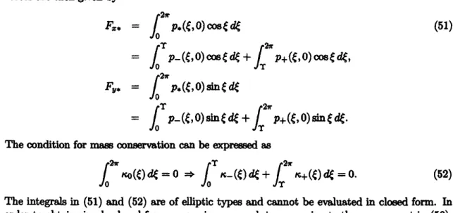
The change of sign $(\pm)$ in (47) gives a dis ntinuity which represents

a

hydraulic jump,

as

illustrated in Fig. 3. Let the jump belocated at $\xi=\prime r,$ $0<\prime r<2\pi$, in terms of the rotating

polar$\infty$ordinatesystemdiscussedinthebeginningofSection 3. Assunuing thatit isnotlocated

at$\xi=0$

or

$2\pi$ (i.e. atthe

sme

location

as

the unbalancemass) givesthe following ‘smoothnaes

condition’ at thispoint;

$\kappa_{0}(0)=\kappa_{0}(2\pi)$

.

(48)

The$\infty nstant\mathcal{A}$

can

bedetemined fromthis condition, whichgives

$\mathcal{A}=\frac{B_{1}}{2}(\frac{A_{1}}{B_{1}})^{2}+x_{*}$

.

(49)

Thesolutionof(45) isthengiven by

Figure3: Sketch of the hydraulicjump solution, eqn. (50).

Let$p\pm(\xi,0)$ be the fluidpressure $\infty rraepondi_{\mathfrak{X}}$tothedepthperturbation $\kappa\pm(\xi)$

.

Thefluid

forces

are

thengivenby

$F_{x*}$ $=$ $\int_{0}^{2n}p.(\xi,0)\infty s\xi\not\in$ (51) $=$ $\int_{0}^{T}p_{-}(\xi,0)m\xi\not\in+\int_{1}^{l\pi}p+(\xi,0)$

oos

$\xi\not\in$,

$F_{y*}$ $=$ $\int_{0}^{2\pi}p_{*}(\xi,0)$stn$\xi d\xi$

$=$ $\int_{0}^{\iota}p_{-}(\xi,0)s\ln\xi d\xi+\int_{r}^{2\pi}p+(\xi,0)\dot{a}n\xi\not\in$

.

The$\infty ndition$for

mass

$\infty nmvation$

can

beexpressed

as

$\int_{0}^{2\pi}\kappa\circ(\xi)d\xi=0\Rightarrow\int_{0}^{T}\kappa_{-}(\xi)d\xi+\int_{r}^{2\pi}\kappa+(\xi)*=0$

.

(52)

The$inte\Psi^{a1_{8}}$in (51) and (52)

are

of elliptic typesandcannot beevaluatedin closedfom. In

order toobtainsimpleclosed-fomexpressions

we

seektoapproximate the squarerootin (50).

As both tems under the square root

are

of the

sme

order of$ni_{\dot{K}}tude$

a

kylorexpansion

doesnot exist.

But by assuming that $x_{r},y_{*}\ll 1$, Lanczoe’s tau method [12]

can

be used. Logarithmic

differentiation of the function $f(x)=\sqrt{x}$gives the differential equation $f’(x)-\#_{l}^{1}f(x)=0$

.

The initial $\infty nditionf(O)=0$

assures

the solution $f(x)=\sqrt{x}$

.

The tau method however

approximates thesolutionvla expansion $\ln$ Chebyshev$polyno\dot{m}\triangleleft s$

.

Retaining onlythe linear

partofthis$\infty ansion$,

we

obtain

$\sqrt{x}\approx\frac{1}{3}(1+2x)$

.

(53)

Equation (50)can thus be apprcximatedas

$\kappa_{0}(\xi)=\kappa\pm(\xi)=\frac{A_{1}}{B_{1}}\pm\frac{1}{3}(\frac{2}{B_{1}})^{\#}\{1+2x_{t}(m\xi-1)+2y_{8}\dot{m}\xi\}$

.

(54)

Using thisexpression the integralsin (51)and (52)

can

be evaluatedinclosed fom. Doing this

we

obtain the$\infty upled$fluid-structureequationsystm

$[-\overline{\omega}_{0}^{2}\{\begin{array}{ll}1+\mu 00 l+\mu\end{array}\}+i\tilde{\omega}_{0}\{\begin{array}{ll}\zeta\overline{\omega}_{0} -2(1+\mu)2(1+\mu) \zeta t\overline{h}\end{array}\}$ (55)

$+$ $\{\begin{array}{ll}\overline{\omega}_{0}^{2}-(l+\mu)\Omega_{*}^{2} -\zeta\Omega_{*}\zeta\Omega_{l} \chi\overline{\omega}_{0}^{2}-(1+\mu)\end{array}\}+\{\begin{array}{ll}\mathfrak{F}_{lx} s_{xy}S_{\Psi} s_{\nu\nu}\end{array}\}]\{\begin{array}{l}x_{*}y_{*}\end{array}\}$

where$\_{xx},$$\ldots,F_{rx},$$\ldots$

are

functionsofthejumplocation $\ell r$,given by

$s_{xx}$ $=$ $-2\mathcal{K}_{1}\{\mathcal{P}_{0(r\prime}-coe’r\dot{m}1^{\cdot}+2\dot{m}^{\prime r\prime}-r+\pi)+\mathcal{P}_{1}(\infty 8^{\prime r_{\sin’}}+r-\pi)\}$ , (56)

$\mathfrak{F}_{xy}$ $=$ $-2\mathcal{K}_{1}(P_{0}-\mathcal{P}_{1})(\cos^{2} T- l)$,

$\mathfrak{F}_{\Psi}$ $=$ _{$-2\mathcal{K}_{1}\{\mathcal{P}_{0}(coe^{2} T- 2coe’r+1)+\mathcal{P}_{1}(1-2\cos^{2}1’)\}$},

$S_{yy}$ $=$ $-2\mathcal{K}_{1}(\mathcal{P}_{0}-\mathcal{P}_{1})(coe$Tsin$\prime r+’r-\pi)$, $\mathcal{F}_{rx}$ $=$ $-2\mathcal{K}_{1}\mathcal{P}_{0}$sin 1,

$F_{ry}$ $=$ $-2\mathcal{K}_{1}\mathcal{P}_{0}(1-\infty s^{\prime r)}$

.

Herein

$\mathcal{P}_{0}$ _$=$ $2(1+2 \delta^{\iota}2\frac{c_{-}}{c_{0}})$ , $\mathcal{P}_{1}=\delta^{2}(\frac{c_{-}}{c_{0}})^{2}$, (57)

$\mathcal{K}_{0}$ _$=$ $\frac{A_{1}}{B_{1}}$, $\mathcal{K}_{1}=\pm\frac{1}{3}(\frac{2}{B_{1}})^{\#}$

The

mass

conservationequation (52) takesthe fom

$2\mathcal{K}_{1}\{(-\dot{m}r-\pi)x_{*}+(coe1^{4}-1)y_{*}\}+\mathcal{K}_{0}\pi+\mathcal{K}_{1}(\pi-r)=0$

.

₍₅₈₎

Foragivenangular velocity$\Omega_{*},$ (55)and (58)_{$cont\dot{m}$}threeequationsfor the

three unknowns

$x_{*},$$y_{*}$, and $r$, which

can

be solvedtogether numerically. [Here, $\mathcal{K}_{0}$issetequal to

zero

in (58).]

In thenumericalexampletofollowwe set $\delta=0.125,$$\mu=0.25,$ $\zeta=13.0,$$\sigma=0.4$, and_$\chi=1.0$

.

InFig. 4,part (a) shows therotoramplitudes$x_{*}$ and$y_{*}$,whilepart (b)shows thejumplocation

(with1 inradians). _{It is noted that the value of the dmping}parameter$\zeta$islarge,whichimplies

the ‘smooth’fom of the $x_{*}$ and$y_{*}$

curves.

Part (b) showsthat the jump is located at $\prime r\approx\pi$for small values ofthe angular velocity $\Omega_{*}$ and that $\prime r$ increases

smoothly with increasingvalueof$\Omega_{*}$, upto $r\approx 4.6$rad. This is not

the way the fluid balanceris expectedto work (see Section 1). The results appear toindicate,

then, _{that mechanismofthe fluid balancermust be}

_one

_or

_more

_solitary

_waves

_{(solitons). This}

remainsto be verified. $x_{*},$$y_{*}$ りさ 15 ハ (a) $\Omega_{*}$ $\prime r$ $0.$

.

_1.5 $\mathfrak{g}$ (b) $\Omega_{*}$

Figure 4: (a)Deflections$x_{*}$ and$y_{*}$ Lower

curve:

$x_{*}$; upper

curve:

$y_{*}$

.

$(b)$ Jumplocation $\prime r$

.

6 Concluding

remarks

Thefluid balancer has been modeled

as

a

rotor partiaUyfilled with fluid. The rotor hastwo degreesof freedom,and thefluidforces acting

on

it

are

evaluatedintemsofshaUowwatertheory.

A simplifled analysis, giving

a

solutionresemblng

a

hydraulicjump,has been

discussed

in

detail.

Itappeaes thatthis solutioncannotrepresent themechanism of thefluid balancer. Futuremork shouldthus$\infty nsider$soliton-type solutions of the Korteweg-de Vries-Burgersequation (37).

References

[1] Nakamura, T., 2009. “Study

on

the improvement of the fluid balanoer of washing $n1\#$

2009, UniversityofCanterbury, NewZealand, pp. $1arrow$

.

[2] Bolotin,V.V., 1963. NonoonservativePrvblems

_of

the Theoiy

_of

Elastic Stability. Pergmon

Press,Oxford.

[3] $Cmda\mathbb{I}$, S.H., 1995. “Rotor dynamics“. In Nonhnear Dynamcsand StochasticMechanics,

W. Kliemann andN. S. Namachivaya, eds., CRC Press, BocaRaton, pp. $1\triangleleft 4$

.

[4] Berman, A. S., Lundgren, T. S., and Cheng, A., 1985. “Asyncronouswhirl in arotating

cylinder partiallyfilled with liquid”. J. FluidMech., 150,pp. 311-$27.

[5] Colding-Jorgensen, J., 1991. “Lmit cycle vibration analysis of a long rotating cylinder

partly filled with fluid”. J.

_of

Eng.

_for

Gas Rrbines andPower, llS, pp. 56k567.

[6] Kasahara, M., Kaneko, S., and Ishii, H., 2000. “Sloehing analysis of

a

$whir\infty$ring”. In

Pror

ofthe $Dynan\dot{u}oe$ and Design Conferenoe 2000, 5-8 August 2000, Japan Soc.

Mech. Eng., pp. 1-6.

[7] $Y\ovalbox{\tt\small REJECT}$, F., 2007. “Self-excited vibration $and\dot{\mu}s$ ofa rotating cylinder partial filled

withliquid (Nonhnear analysisbyshallow watertheory)“. $\eta_{uns}$

.

Japan Society

of

Mech.

Eng. (C), $7S(735)$,pp. 28-37.

[8] Green, K.,Chmpneys, A.R.,andLieven, N. J.,2006. “Bifurcation$ga1\dot{\mu}s$of

an

automatic

dynamic balancing mechanismfor$\infty entric$rotors”. J. Sound Vib., 291, pp. 861-881.

[9] Whithm,G. B., 1999. Lin

ear

ard Nonlinear Waves. Wiley-Interscience, NewYork, NY.

[10] $Pet\infty v\mathbb{A}\ddot{u}$, S. V., 1999. “Exact solutions ofthe foroed Burgers equation”. Tech. Phys.,

44(8), pp. 87&881.

[11] Smyth, N.F., 1987. “Modulationtheorysolution forresonant flow

over

topography”. Proc.

R. Soc. Lond. A, 409,pp. 79-97.