The Heegaard Floer complexes of a trivalent graph defined on two Heegaard diagrams (Intelligence of Low-dimensional Topology)

全文

(1)69. The Heegaard Floer complexes of a trivalent graph defined on two Heegaard diagrams Yuanyuan Bao Graduate School of Mathematical Sciences, the University of Tokyo. 1. Introduction. In the report, let G denote an embedded oriented connected trivalent graph in S^{3} without source or sink. Namely each vertex of G is one of the following two cases.. or. Figure 1: Vertices of G.. Choose a generic point. \delta. G. in. and assign a coloring. c. on. G.. Then we consider the. Heegaard Floer complex CFG(G, \delta, c) . The homology of CFG (G, \delta, c) , which is denoted by HFG(G, \delta, c) , is a topological invariant of G with the choice of \delta and c. In this report, we consider two types of Heegaard diagrams, which have both been. studied in [5] for singular knots. We extend the constructions to the case of trivalent graphs and study the Heegaard Floer complexes CFG(G, \delta, c) defined on them.. For the Heegaard diagram of type one, which is given in Example 2.2, we generalize. the results in [5]. This part is a joint work with Zhongtao Wu. Let \mathbb{F}=\mathbb{Z}/2\mathbb{Z} . Let C(G, \delta, c) be the \mathb {F}‐vector space. \bigoplus_{x\inS(G\delta)},\bigotimes_{e\inE_{x}(\frac{\mathb {F}[U_{e}] {U_{e}^{c(e)}=0}) ,. where S(G, \delta) is the set of Kauffman states, E_{x} is a subset of edges of. G. associated. \mathcal{A}‐grading. with and U_{e} is the variable corresponding to an edge . We define the and \mathcal{M} ‐grading of a Kauffman state by using the local contributions in Figures 6 and 7, and x. e. extend them to gradings of C(G, \delta, c) by adding the rules \mathcal{A}(U_{e})=-c(e) and \mathcal{M}(U_{e})=0. Theorem 1.1 (B. and Wu). Let C_{d}(G, \delta, c;s) be the F ‐vector space generated by the generators of C(G, \delta, c) with \mathcal{A} ‐grading s and \mathcal{M} ‐grading d . Then there is a differential \partial :. C(G, \delta, c;s)arrow C(G, \delta, c;s). that carries C_{d}(G, \delta, c;s) to C_{d-1}(G, \delta, c;s) satisfying H_{d}(G, \delta, c;s)\cong HFG_{d}(G, \delta, c;s) ..

(2) 70 Note that \mathcal{A}‐grading and \mathcal{M} ‐grading for a Kauffman states correspond to the Alexander grading and Maslov grading of the original chain complex. As a corollary of Theorem 1.1, we get the following formula for the Euler characteristic.. Let \triangle_{(G,c)}(t) be the Alexander polynomial defined in [3], which is defined up to a factor. of \pm t^{k} for k\in \mathbb{Z} . We say f(t)=g(t) if f(t)=\pm t^{k}g(t) for some k\in \mathbb{Z}.. Corollary 1.2 (B. and Wu).. \chi(HFG(G, \delta, s))=[\delta]\triangle_{(G,c)}(t) ,. (1). where [\delta] is a factor related to the position of \delta.. For a plane trivalent graph, we have the following result.. Corollary 1.3 (B. and Wu). Suppose G is a plane trivalent graph. Then the group HFG(G, \delta, c) is determined by the Alexander polynomial \triangle_{(G,c)}(t) ; indeed, the homology HFG (G, \delta, c) is supported on the zero Maslov grading level. The Heegaard diagram of type two is given in Example 2.4.. The results on this. Heegaard diagram were written in [2], which has been submitted for publication, so we briefly summarize the results in Section 4.. Acknowledgement: This work was partially supported by the Research Institute for. Mathematical Sciences, an International Joint Usage/Research Center located in Kyoto University. 2. Preliminaries. 2.1. Heegaard diagram. Suppose G is a connected trivalent graph. Let V be the set of vertices of G and E be the set of edges of G . Suppose |V|=n and |E|=m . Choose a generic point on G and call it \delta . It is convenient to regard \delta as a new bivalent vertex of G . The Heegaard diagram of. (G, \delta) is defined as follows, which was proposed in [1]. Definition 2.1. A quintet (\Sigma, \alpha, \beta, w, z) is called a Heegaard diagram for (G, \delta) if it satisfies the following conditions. 1. (\Sigma, \alpha, \beta, w) is an (n+1) ‐pointed Heegaard diagram for S^{3} , and points in \Sigma\backslash (\alpha\cup\beta\cup w) .. 2. For each vertex v\in V\cup\{\delta\} whose indegree is s=1. or 2 ) , there exists a smooth embedding. (\Sigma\backslash \alpha, w, z) (resp. \psi_{v} :. \varphi_{v}. l=1. :. z. is a set of (m+1). or 2 (resp.. outdegree is. (L_{1}ol2 , \{0\}, \{1,2, , l\})\simeq+. (L_{1}o82 , \{0\}, \{1,2, \cdots , s\})\simeq+*(\Sigma\backslash \beta, w, z) ). so that the im‐. ages of \varphi_{v} (resp. \psi_{v} ) are pairwisely disjoint and \bigcup_{v\in V\cup\{\delta\}}({\rm Im}(\varphi_{v})\cup{\rm Im}(\psi_{v}) recovers G , when we push the interior of {\rm Im}(\varphi_{v}) (resp. {\rm Im}(\psi_{v}) ) slightly into U_{\alpha} (resp. U_{\beta} ). Here U_{\alpha} (resp. U_{\beta} ) is obtained from \Sigma by attaching 2‐handles along \alpha ‐curves (resp. \beta ‐curves)..

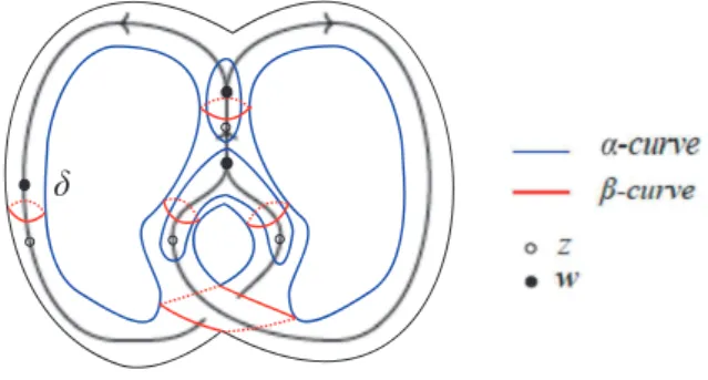
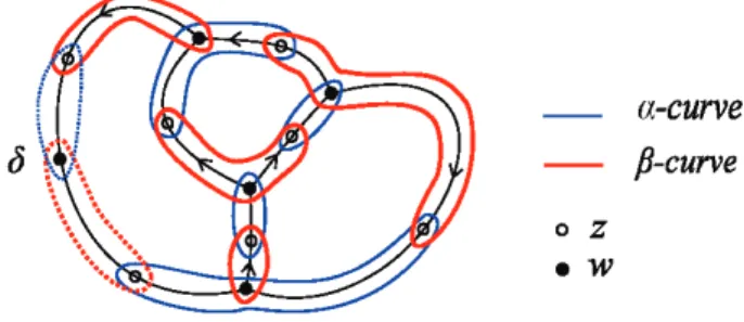
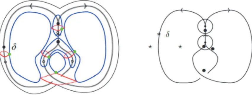
(3) 71 71 From the definition it is easy to see that on the Heegaard diagram \Sigma , we assign a base point w_{v} around a vertex and a basepoint z_{e} at an edge e of G , and the base points w_{\delta} and z_{\delta} around \delta . In this report, we focus on two types of Heegaard diagrams. Here we introduce them as examples.. Example 2.2 (Heegaard diagram of type one). This Heegaard diagram was introduced in [1], which extended the construction in [5]. Consider a graph diagram D\subset \mathbb{R}^{2} for a given graph G\subset S^{3}.. 1. Regard D as a 1‐complex in S^{3} and take a tubular neighbourhood of it in S^{3} . It is a handlebody and its boundary is the Heegaard surface \Sigma. 2. The diagram D divides \mathb {R}^{2} into several regions. For each bounded region, introduce an \alpha ‐curve on \Sigma which encloses the region.. 3. For each crossing of. D,. 4. Place the base point. w_{v}. introduce a \beta ‐curve as shown in Figure 2. on each vertex v\in V.. 5. For a vertex v\in V with indegree l=1 or 2, introduce l\beta ‐curves which are meridians of the edges pointing to v and l base points of type z on the edges pointing to v. Introduce an. \alpha ‐curve. points of type. z. \alpha_{v} which bounds a disk in \Sigma that contains w_{v} and all the base. on the edges pointing to. v.. 6. For \delta , introduce a \beta ‐curve which is the meridian of the edge containing duce two base points w_{\delta} and z_{\delta} around \delta.. \delta. and intro‐. a-c\iota m\cdot e. \beta_{-Cl}n\cdot e 0-\bullet 1t. ’. Figure 2: The Heegaard diagram of type one associated with a graph diagram.. Remark 2.3. Example 2.2 was first proposed in [1], where we studied bipartite graphs. A trivalent graph without source or sink can be regarded as a perticular bipartite graph.. Example 2.4 (Heegaard diagram of type two). We consider the second type of Heegaard diagram only for plane graphs. It extends the construction in [5] for a singular knot. G.. For a plane oriented graph G without source or sink, choose a point We introduce a Heegaard diagram for (G, \delta) as follows.. \delta. on an edge of.

(4) 72. — —. a‐curve. \beta‐curve. oz ew. Figure 3: A Heegaard diagram for G with a point 6.. ı. The Heegaard surface is S^{2} where G is embedded as a plane graph.. 2. At each vertex v\in V , introduce a base point a base point z_{e}. 3. For \delta , introduce two base points. 4. Around each vertex. v\in V ,. w_{\delta}. and. z_{\delta}. w_{v}. , and on each edge. e. of. G. introduce. around \delta.. introduce a curve. a_{v}. which encloses the base point. w_{v}. at. and the base point(s) z(' s) on the edge(s) pointing to v . Introduce a curve \beta_{v} which encloses the base point w_{v} at v and the base point(s) z(' s) on the edge(s) pointing v. out of. v.. As a result, we get the following data H=(S^{2}, \{\alpha_{v}\}_{v\in v}, \{\beta_{v}\}_{v\in v}, w, z) , which is a Hee‐ gaard diagram for (G, \delta) . See Fig. 3 for an example. 2.2. The Heegaard Floer complex. Let (\Sigma,a,\beta, w, z) be a Heegaard diagram for a graph (G,\delta) whose number of a‐curves (and also \beta‐curves) is d . Let \Gamma_{\alpha}=\alpha_{1}x\alpha_{1}\cross. \cross\alpha_{d} and. T_{\beta}=\beta_{1}\cross\beta_{1}\cross. \cross\beta_{d}. Sym^{d}(\Sigma) . Given x,y\in\Gamma_{\alpha}\cap T_{\beta} , let \pi_{2}(x,y) be the set of relative homology classes of Whitney disks from x to y with boundary in \Gamma_{\alpha} and \Gamma_{\beta} . For \phi\in\pi_{2}(x, y) , let \mu(\phi) be its Maslov index and \hat{\mathcal{M} (\phi) be the moduli space of pseud (\succ holomorphic disks in the class \phi modulo \mathbb{R}. Let D_{1}, D_{2} , , D_{h} denote the closures of the components of \Sigma\backslash (a\cup\beta). A domain is a 2‐chain on \Sigma of the form D= \sum_{i=1}^{h}a_{i}D_{i} , where a_{i}\in \mathbb{Z} is called the local multiplicity of D at D_{i} . For a point p in the interior of D_{i} , let n_{p}(D) denote the local multiplicity of D at the point p , which equals a_{*}\cdot . A domain D is a positive domain if a_{1}\geq 0 for 1\leq i\leq h. A domain P= \sum_{i=1}^{h}a_{i}D_{i} is called a periodic domain if \partial P is a &‐linear combination of be the tori in the symmetric product. and \beta ‐curves and P\cap w=P\cap z=\emptyset. To each base point z_{e} , we assign a variable U_{e} . We define the chain complex C\Gamma G(G, \delta) to be the free \Gamma[\{U_{e}\}_{e\in E}] ‐module generated by \Gamma_{\alpha}\cap\Gamma_{\beta} , where \Gamma=\mathbb{Z}/2\mathbb{Z} . Note that the generating set \Gamma_{\alpha}\cap\Gamma_{\beta} has a one‐to‐one correspondence with the set a ‐curves. S=\{ (x_{1},x_{2}, \cdots , x_{d})|x_{i}\in\alpha_{i}\cap\beta_{\sigma(:)}, 1\leq i\leq d,\sigma\in S_{d}\}..

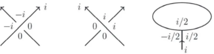
(5) 73 Therefore Then. S. is also regarded as the generating set.. CFG(G, \delta). is endowed with the differential. \partial(x)=\sum_{y\in\Gam a_{\alpha}\cap \mathb {T}_{\beta} \sum_{2\{\phi\ n\pi(x,y)|\mu(\phi)=1,n_{w}(\phi)=\{0\},n_{z_{\delta} (\phi)=0\} \#\hat{\mathcal{M} (\phi)\cdot(\prod_{e\in E}U_{e}^{n_{z_{e} (\phi)} \cdot y , where. (2). n_{w}(\phi)=\{n_{w}(\phi)|w\in w\}.. To simplify the discussion, we further endow a coloring to G. A balanced coloring is a map c:Earrow \mathbb{Z}_{\geq 0} such that for each vertex v of G,. \sum c(e)= \sum c(e). e. Let. c(v). : pointing into. v. e. : pointing out of. be the value above.. Definition 2.5. The relative Alexander grading. for. x,. .. v. A. and Maslov grading. M. are as follows:. A(x)-A(y)= \sum_{v\in V}c(v)\cdot n_{w_{v} (\phi)-\sum_{e\in E}c(e)\cdot n_{z_{e} (\phi) ,. (3). M(x)-M(y)= \mu(\phi)-2\sum_{v\in V\cup\{\delta\}}n_{w_{v} (\phi) ,. (4). y\in \mathbb{T}_{\alpha}\cap \mathbb{T}_{\beta} , where \phi\in\pi_{2}(x, y) .. The functions A and N defined above induce on CFG(G, \delta) , the Alexander and Maslov gradings, with the convention that. A(U_{e})=-c(e) , M(U_{e})=0. The differential. \partial. drops the Maslov grading by one, and preserves the Alexander grading.. Proposition 2.6. The homology of CFG(G, \delta, c) is a topological invariant of with the choice of \delta and c.. 3. G. together. Heegaard Floer complex: type one. The purpose of this section is to prove Theorem 1.1 and Corollaries 1.2 and 1.3. 3.1. Kauffman states. We recall the definition of Kauffman states, which was described in detail in [3]. Definition 3.1. Starting from a trivalent graph diagram (D, \delta) , we can obtain a decorated diagram (D, \delta) by drawing a circle around each vertex of D. 1. Cr(D) : denotes the set of crossings, including the types. \near ow^{\backslash }\backslash and_{/}\backslash '. which are the. double points of the diagram and the type \varphi which are the intersection points around each vertex between the incoming edges with the circle..

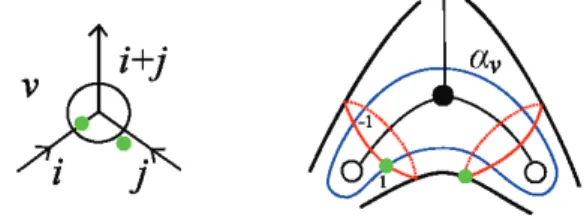
(6) 74 2. {\rm Re}(D) : denotes the set of regions, including the regular regions of \mathb {R}^{2} separated by D and the circle regions around the vertices. Marked regions are the regions adjacent to the base point \delta , and the others are called unmarked regions.. \near ow_{\backslash }^{\backslash }or\backslash _{/}' , there are four corners around it, and we them the north, south, west, and east corners of the crossing. Around a crossing of type \varphi there are three corners, and we call the one inside the circle region the north corner, the one on the left of the crossing the west corner and the one on the right the east corner. Note also that every corner belongs to a unique region in. 3. Corners: For a crossing of type c\ovalbox{\t \smal REJECT}. {\rm Re}(D). .. Calculating the Euler characteristic of \mathb {R}^{2} using. D. gives. |{\rm Re}(D)|=|Cr(D)|+2. The point \delta is chosen so that it is adjacent to two distinct regions, which will be denoted by R_{w} and R.. Definition 3.2. A Kauffman state, or simply, a state for a decorated diagram (D, \delta) is a bijective map. x:Cr(D)arrow{\rm Re}(D)\backslash \{R_{w}, R_{v}\},. which sends a crossing in Cr(D) to one of its corners. Denote S(D, \delta) the set of all states. For each Kauffman state x , around each vertex v there is a unique edge the crossing on which is sent to the circle region. Let E_{x} be the set of such edges. Consider the Heegaard diagram in Example 2.2. We see that each Kauffman state is associated to 2^{n} different generators in \Gamma_{\alpha}\cap\Gamma_{\beta} , where n is the number of vertices. More precisely, each intersection point in T_{\alpha}\cap\Gamma_{\beta} is represented by a pair (x, \epsilon_{x}) , where x is a. Kauffman state and. \epsilon_{c}. :V. Figure 4: The internal curve. a_{v}. arrow. { \pm ı}.. intersects the same \beta ‐curve at two points, which we label them as 1 and. -1.. Suppose x+ and x_{-} are two generators which are identical except that around the vertex v, x_{+} is labeled by ı and x_{-} is labeled by -1 . There is a bigon connecting x_{-} to x_{+} which contains a base point z_{e} . Then we have. A(x_{-})-A(x_{+})=-c(e)\leq 0..

(7) 75. Figure 5: A kauffman state and its corresponding Alexander grading maximizer.. Therefore among all the intersection points in \mathb {T}_{\alpha}\cap \mathb {T}_{\beta} which corresponds to the same Kauffman state x , the one with \epsilon_{x}(v)=+1 is the unique intersection point that has maximal Alexander grading. We call it the Alexander grading maximizer of the state x.. For each regular region in {\rm Re}(D) , we recall the definition of its index Ind(\cdot) in [3],. which was defined as follows.. 1. The index of the unbounded region is set to be. 0.. 2. The indices of the other regular regions are inductively determined by the rule as exhibited below: when an edge with color i points upward, let the difference of the index of its left‐hand side region and that of its right‐hand side region be i. i n n-i. The definition of a balanced coloring guarantees that the above rules give rise to a well‐defined index for each regular region.. Definition 3.3. Suppose \delta is on an edge with color i , and the indices of the regions adjacent to \delta are n and n-i . Define. |\delta|=t^{n-i}-t^{n} 3.2. and. [\delta]=(t^{-1/2}-t^{1/2})^{-1}|\delta|.. Alexander grading. Lemma 3.4. Let x, y be two Kauffman states and let maximizers that correspond to them. Then we have. \mathcal{A}(x)-\mathcal{A}(y)=A(x)-A(y) where. \mathcal{A}(x)=\sum_{c\in Cr(D)}\mathcal{A}_{c}^{x(c)}. x, y. be the Alexander grading. ,. is calculated using the local contribution in Figure 6..

(8) 76. Figure 6: The local contribution. \mathcal{A}_{c}^{\triangle}.. Proof. The proof is similar with the proof of Lemma 4.2 in [5]. For show that any homology class \phi\in\pi_{2}(x, y) satisfies. x. \mathcal{A}(x)-\mathcal{A}(y)=\sum_{v\in V}c(v)\cdot n_{w_{v} (\phi)- \sum_{e\in E}c(e)\cdot n_{z_{e} (\phi) Around each vertex v , let v\Leftrightar ow be the oriented simple arc from. surface for each edge. w_{v}. to. .. z_{e}. on the Heegaard. be the inverse of v‐2. Suppose each arc v‐2 intersects transversely with the boundary of \phi . For an intersection point p\in\overline{v}2\cap\partial\phi (or evarrow\cap\partial\phi) , define \# p=(-1)^{sign(p)}c(e) e. adjecent to , and. and y , It suffices to. v. \frac{}{e[j}. to be the algebraic intersection number of \overline{v}2 (or. \frac{}{elj} ) and \partial\phi at p , where sign(p) is +1 if the orientation of the intersection agrees with the orientation of the Heegaard surface and -1 otherwise.. Around a vertex. v. of. G,. let. \eta_{v}. be the union of. \frac{}{vt},s. \theta_{v} be the union of \frac{}{e\prime[j},s for all the edges pointing to. v. for those edges e pointing to v . Let and \overline{v}2 ’s for all the edges leaving v.. Then we have. A(x)-A(y) = \sum_{v\in V}\#(\eta_{v}\cap\partial\phi) = \sum_{v\in V}\#((\eta_{v}+\theta_{v})\cap\partial\phi). .. The first equality follows from the definition of A(x)-A(y) and the fact that \phi is a 2‐complex on the Heegaard surface. The second equality follows from the facts that U_{v}\theta_{v} replicates G and c is a balanced coloring defined on G . Namely \sum_{v\in V}\#(\theta_{v}\cap\partial\phi)=0. Let \beta_{c} be the \beta ‐curve around a double crossing c , and \alpha_{v} be the internal \alpha ‐curve around a vertex v . For \alpha ‐curves, the only ones that intersect (\eta_{v}+\theta_{v}) are the internal \alpha_{v} ’s around vertices, and the only \beta ‐curves that algebraically intersect (\eta_{v}+\theta_{v}) are those \beta_{c}' s . Note that \partial\phi are union of arcs on \alpha\cup\beta . Therefore we have. \sum\#((\eta_{v}+\theta_{v})\cap\partial\phi). v\in V. = \sum\#((\eta_{v}+\theta_{v})\cap\partial\phi|_{\alpha_{v} )+ \sum \#[(\bigcup_{v}\theta_{v})\cap\partial\phi|_{\beta_{c} ]. v\in V. c. : doubıe crossing.

(9) 77 We claim that. \#((\eta_{v}+\theta_{v})\cap\partial\phi|_{\alpha_{v}}) = \mathcal{A}_{v}^{x(v) }-\mathcal{A}_{v}^{y}(v)+[Ind(x(v))-Ind(y(v))] , \#[(\bigcup_{v}\theta_{v})\cap\partial\phi|_{\beta_{c}}] = \mathcal{A}_{c} ^{x(c)}-\mathcal{A}_{c}^{y(c)}+[Ind(x(c))-Ind(x(c))] ,. (5) (6). where \mathcal{A}_{v}^{x(v)} is the sum of the local contributions around v for the state x , and Ind(x(v)) is the sum of the indices of the regular regions occupied by x around v . For each vertex v , the intersection number of (\eta_{v}+\theta_{v}) with the internal \alpha_{v} is zero. For each \beta_{c} , the. intersection number of ( \bigcup_{v}\theta_{v}) with it is also zero. Therefore it suffices to verify (5) and (6) by choosing any arc connecting x to y on the internal \alpha_{v} ’s and \beta_{c}' s. We consider all the possible locations of. x. and. y. around a vertex and around a crossing. to verify (5) and (6). It is easy to see that all the possible locations can be obtained as compositions of the six cases in Tables 1 and 2.. Now summing equations (5) and (6) we have. A(x)-A(y)=[ \mathcal{A}(x)+\sum_{c\in Cr(D)}Ind(x(c) ]-[\mathcal{A}(y)+ \sum_{c\in Cr(D)}Ind(y(c) ]. On the other hand, we see that. \sum_{c\in Cr(D)}Ind(x(c) =\sum_{c\in Cr(D)}Ind(y(c). ,. which is the sum of indices over all unmarked regular regions of D.. Table 1: Verify Eq. (5) around a vertex.. 3.3. Maslov grading. For the Maslov grading, we can also calculate it locally as below.. \square.

(10) 78. Table 2: Verify Eq. (6) around a double crossing.. Figure 7: The local contribution. Lemma 3.5. Let x be a Kauffman state and let that corresponds to it. Then we have. where. \mathcal{M}(x)=\sum_{c\in Cr(D)}\mathcal{M}_{c}^{x(c)}. be the Alexander grading maximizer. x. \mathcal{M}(x)=M(x). \mathcal{M}_{c}^{\triangle}.. ,. is calculated using the local contribution in Figure 7.. The proof in [5] can be generalized trivially to our case. In the proof of [5], only four‐ valent vertices (singular crossings) are considered. However, the proof works for graphs which contains both trivalent and four‐valent vertices.. For the readers’ convenience, we summarize the sketch of the proof and point out the notational differences. Note that the definition of M(x) does not depend on the z base points and the coloring c . Suppressing the z base points, we get an (n+1) ‐pointed Heegaard diagram for S^{3}. Let G be a plane trivalent graph. Two Kauffman states are said to be equivalent if they coincide with each other inside the circle regions. This definition is an adaption of. Definition 4.3 [5] to our situation. By using exactly the same argument, we could prove. that two Kauffman states are equivalent if and only if they are the same state.. Following the discussion in Proposition 4.6 of [5], we can show the following fact. Let (G, \delta) be a plane trivalent graph. Suppose x is a Kauffman state and x is the corresponding Alexander maximizer. Then we have M(x)=0. Now we consider a general trivalent graph (G, \delta) . Consider the Heegaard diagram.

(11) 79 of type one H=(\Sigma, \alpha, \beta, w) for (G, \delta) , where. is suppressed. Consider a Kauffman. z. for (G, \delta) . Then following the recipe in the proof of Theorem 4.1 of [5], one can construction a new Heegaard diagram H_{x}=(\Sigma, \gamma, \beta, w) , which deeply depends on x . It is an (n+1) ‐pointed Heegaard diagram for S^{3} . Then we can show that the generators state. x. induced from x are the only generators for H_{x} , the number of which is 2^{n} . Namely the differential of the chain complex defined on H_{x} is trivial. Let x be the Alexander maximizer of x in H=(\Sigma, \alpha, \beta, w) , and let x' be the induced generator on H_{x} . Then we have. M(x')=0.. On the other hand, H_{\alpha,\gamma}=(\Sigma, \alpha, \gamma, w) is a Heegaard diagram for (S^{1}\cross S^{2})^{\# d} , where d is the cardinality of \alpha . The differential defined on H_{\alpha,\gamma} is also trivial. Suppose \theta is the generator with maximal Maslov grading, which is M(\theta)=0. Consider the homological triangle connecting x, x' and \theta . One can finally show that M(x)=n-p , where n is the number of negative crossings whose images under x are north corners and p is the number of positive crossings whose images under x are north corners. It is indeed the conclusion we want to show in Lemma 3.5. 3.4. Proof of Theorem 1.1.. The proof follows the idea in the proofs of Proposition 4.6 and Theorem 4.1 in [5]. Since. G. is connected, we have the following lemma.. Lemma 3.6. Let P be a periodic domain in the Heegaard diagram H=(\Sigma, \alpha, \beta, w) of type one. If n_{z}(P)=n_{w}(P)=\{0\}, P is a trivial domain. Using the lemma above, we can define a filtration on CFG(G, \delta, c) . Consider all the regions of \Sigma\backslash (\alpha\cup\beta) , and place a point in each region disjoint from z_{e}' s . Let Q be the set of such points.. Definition 3.7. We define a partial order \mathcal{K} on \mathbb{F}[\{U_{e}\}_{e\in E}]\langle \mathbb{T}_{\alpha}\cap \mathbb{T} _{\beta} }. For two elements a, b\in \mathbb{F}[\{U_{e}\}_{e\in E}]\langle \mathbb{T}_{\alpha}\cap \mathbb{T}_ {\beta}\rangle , if there is a domain \phi connecting a to b with n_{w}(\phi)=\{0\} and n_{z_{\delta}}(\phi)=0 , let \mathcal{K}(a)-\mathcal{K}(b)=\#_{alg}(\phi\cap Q) ,. where the right hand side denotes the algebraic intersection number of \phi and Q. The partial order. K. is well‐defined since by Lemma 3.6 if the domain \phi exists, it is. unique.. Lemma 3.8. For have. a,. b\in \mathbb{F}[\{U_{e}\}_{e\in E}]\{\mathbb{T}_{\alpha}\cap \mathbb{T}_{\beta} \} , suppose \mathcal{K}(b)\leq \mathcal{K}(a). Namely. \mathcal{K}. b. is a summand in \partial(a) . Then we. .. induces a filtration on (CFG (G, \delta, c), \partial ).. Proof. The pseudo‐holomorphic disk \phi connecting section number with Q.. a. to. b. always has non‐negative inter‐ \square.

(12) 80 Proof of Theorem 1.1. For a Kauffman state x , let x_{+} and x_{-} are two generators corre‐ sponding to x which are identical except around a base point z_{e} . Then the bigon containing z_{e} connects x_{-} to x+\cdot Its homology class \phi admits a single holomorphic representative up to reparameterization. The differential on the E_{0} page of CFG(G, \delta, c) under the filtration \mathcal{K} counts only those bigons described above. Namely it only connects generators which have common underlying Kauffman state. Therefore the chain complex on the E_{0} page splits along the set S(G, \delta) . For each Kauffman state x , the chain complex on the E_{0} page is the tensor product of the chain complexes of the form. \mathbb{F}[\{U_{e}\}_{e\in E}]ar ow^{U_{e}^{c(e)} \mathbb{F}[\{U_{e}\}_{e\in E} ], for e\in E_{x} . The cokernal of each such short differential is generated as a \mathb {F}‐vector space by \{x_{+}, U_{e}\cdot x_{+}, \cdot\cdot\cdot , U_{e}^{c(e)-1}\cdot x_{+}\}. The E_{1} page is now a free module generated by Kauffman states. More precisely, as a \mathb {F} ‐vector. space, it is. \bigoplus_{x\inS(G\delta)},\bigotimes_{e\inE_{x}(\frac{\mathb {F}[U_{e}] {U_{e}^{c(e)}=0}). .. \square. Now we prove Corollaries 1.2 and 1.3.. Proof of Corollary 1.2. We elaborate the proof here by looking back at the differential \partial_{0} in E_{0}|‐page in the proof of Theorem 1.1. The differential given by the bigon that passes z_{e}. is of the form. \partial_{0}x_{-}=U_{e}^{c(e)}\cdot x_{+}, from which we see that the cokernal is generated by \{x_{+}, U_{e}\cdot x_{+}, , U_{e}^{c(e)-1}\cdot x_{+}\} . There are a total of c(e) number of generators with the same Maslov grading and different Alexander gradings, which contribute a factor. 1+t+ \cdots t^{c(e)-1}=[c(e)]\cdot t\frac{c(e)-i}{2}. \dot{ \imatgures h} n[3],weobta\6dot{ \imath} ntheident\dot{ \imath} ficat\dot{ \imath} on.\square aroundz_{e}fions ore\in E_{x},where[k]:=\frac{t^{k/2}- t^{-k/2} {t^{1/2}-t^{-1/2},tr\dot{ \imathocal } bu}.Final1contributions ybycompar\dot{ \imath} ngthel. \dot{ \imath} nF\dot{ \imath}. and7andthe1oca1cont. Proof of Corollary 1.2. When G is a plane trivalent graph, all the generators in Theorem \square 1.1 have zero \mathcal{M} ‐grading. Hence, the differential on the chain complex is trivial.. 4. Heegaard Floer complex: type two. We consider a plane trivalent graph G . Viro in [6] proposed a vertex state sum formula for the gl(1|1) ‐Alexander polynomial. Choose a point \delta on an outermost edge of G. A Viro state is a map s : Earrow\{0,1\} which sends the edge containing \delta to zero and satisfies the condition that at each vertex, the sum of s(e) for all the edges e pointing toward the.

(13) 81 81 vertex equals that for the edges pointing out of the vertex. Let S be the set of states. By definition, around each vertex we have the following six possibilities under a state, where the dotted edges are those which are sent to zero and the solid edges are those which are sent to one.. r. . .\{\near ow \nwarow_{t}.\cdot\cdot\cdot\cdot\cdotN Consider the intersection points of T:=. \alpha. \backsla h\cdot\cdot(\nwarow \near ow 1_{r}. .. ‐curves and \beta ‐curves. Let. { \{x_{v}\}_{v\in V}|x_{v}\in\alpha_{\sigma(v)}\cap\beta_{v} for a bijection. \sigma. of. V }.. Let \sigma_{x} be the bijection that defines x\in T . It is easy to see that the intersection points always appear in pairs around a base point. Two elements x=\{x_{v}\}_{v\in V} and y=\{y_{v}\}_{v\in V} are said to be equivalent (x\sim y) if x_{v} and y_{v} are around the same base point for any v\in V . Let [x] be the equivalence class of x . It is obvious that \sigma_{x} keeps invariant within the equivalence class of x. Our first result is:. Proposition 4.1. There is an identification between T/\sim and S. The gl(1|1) ‐Alexander polynomial is defined by assigning Boltzmann weights to each vertex under each state as follows. The Boltzmann weights were originally obtained by scaling the Clebsch‐Gordan morphisms for irreducible U_{q}(gl(1|1)) ‐modules of dimension. (1 | 1).. Our second result is:. Proposition 4.2. The Boltzmann weights around trivalent vertices, which determine. the gl(lll)‐Alexander polynomial, can be obtained from the Fox calculus on the Heegaard diagram of type two. References. [1] Y. BAO, Heegaard floer homology for embedded bipartite graphs, arXiv:1401.6608v3 (2016). [2] —, A topological interpretation of Viro’s gl (l |1) ‐Alexander polynomial of a graph, arXiv:1801.06301 (2018)..

(14) 82 [3] Y. BAO AND Z. WU, An Alexander polynomial for MOY graphs, arXiv: 1708.09092 (2018). [4] L. H. KAUFFMAN, Formal knot theory, vol. 30 of Mathematical Notes, Princeton University Press, Princeton, NJ, (1983).. [5] P. OZSVÁTH, A. STIPSICZ AND Z. SZABÓ, Floer homology and singular knots, J. Topology 2 (2009) 380‐404. [6] O. Viro, Quantum relatives of the Alexander polynomial, Algebra i Analiz, 18 (2006) 63‐157.. Graduate School of Mathematical Sciences. the University of Tokyo 3‐8‐1 Komaba, Meguro‐ku, Tokyo 153‐8914 JAPAN. E‐‐mail address: [email protected]‐tokyo.ac.jp.

(15)