Global and local structures of oscillatory bifurcation diagrams (Succession and Innovation of Studies on ODEs in Real Domains)

全文

(1)147. 数理解析研究所講究録第2080巻 2018年 147-156. Global and local structures of oscillatory bifurcation diagrams 広島大学大学院工学研究科柴田徹太郎 (Tetsutaro Shibata) Graduate School of Engineering Hiroshima University. 1. Introduction. We first consider the following example of nonlinear eigenvalue problems. -u''(t) = $\lambda$(u(t)+g(u(t))) , t\in I=:(-1,1) ,. (1.1). u(t) > 0, t\in I ,. (1.2). u(-1) = u(1)=0 . Here, g(u). (1.3). :=\displaystyle \frac{1}{2}\sin^{k}u(t) , k\geq 1 is a given integer, and. $\lambda$>0. is a bifurcation parameter. We. know from [15] that the solution set of (1.1)-(1.3) consists of the set Q. :=. { ( $\lambda$(k, $\alpha$) , u_{ $\alpha$} ) | sol. of (1.1)-(1.3) with \Vert u_{ $\alpha$}\Vert_{\infty}= $\alpha$ } \subset \mathbb{R}_{+}\times C^{2}(\overline{I}) .. Indeed, in this case, for any given. (1.3) with. $\alpha$. =. \Vert u_{ $\alpha$}\Vert_{\infty} and. $\lambda$. $\alpha$>0 ,. there exists a unique solution pair ( $\lambda$, u_{ $\alpha$}) of (1.1)-. is parameterized by. consider the asymptotic behavior of $\lambda$(k, $\alpha$) as. $\alpha$. . So we write as. $\alpha$\rightarrow\infty. $\lambda$. =. $\lambda$(k, $\alpha$) . If we. , then it seems clear that. $\lambda$(k, $\alpha$)\displaystyle\rightar ow\frac{$\pi$^{2}{4} .. (1.4). $\lambda$. $\pi$^{2}. (2n, $\alpha$) 2010 AMS Subject Classifications: Primary 34\mathrm{F}10 This work was supported by JSPS KAKENHI Grant Number. \mathrm{J}\mathrm{P}17\mathrm{K}05330..

(2) 148. $\lambda$. $\pi$^{2}. \downarrow(2n+1, $\alpha$) So it is natural to expect that the rate of convergence of $\lambda$(2n, $\alpha$) to $\pi$^{2}/4 as. $\alpha$\rightarrow\infty. is the. same as that of $\lambda$(2n+1, $\alpha$) . However, we will find that the following formula holds.. | $\lambda$(2n_{1}+1, $\alpha$)-$\pi$^{2}/4| \ll| $\lambda$(2n_{2}, $\alpha$)-$\pi$^{2}/4|\rightarrow 0 , where. n_{1}. \geq 1. and. n_{2}. \geq 1. (1.5). are arbitrary given integers. To show (1.5), we calculate the. asymptotic behavior of $\lambda$(k, $\alpha$) precisely.. Theorem 1.1 ([19]). (i) Let. k=2n. (n\geq 1) . Then as. $\alpha$\rightarrow\infty. $\lambda$(2n, $\alpha$)=\displayst le\frac{$\pi$^{2}{4}-\frac{$\pi$}{2^{2n+1}$\alpha$}\left(\begin{ar y}{l 2n\ n \end{ar y}\right)-\frac{$\pi$^{3/2}{2^{2n+1}$\alpha$^{3/2}\sum_{r=0}^{n-1}(-1)^{n-r}\left(\begin{ar y}{l 2n\ r \end{ar y}\right) \displaystyle \times\frac{1}{\sqrt{n-r} \sin( 2n-2r) $\alpha$+\frac{ $\pi$}{4})+O($\alpha$^{-2}) .. (ii) Let. k=2n+1. (n\geq 0) . Then as. (1.6). $\alpha$\rightarrow\infty. $\lambda$(2n+1, $\alpha$) = \displaystyle \frac{$\pi$^{2} {4}-\frac{$\pi$^{3/2} {2^{2n+1}$\alpha$^{3/2} \sum_{r=0}^{n}(-1)^{n+r}\left(2n & +1r\right). (1.7). \displaystyle \times\sqrt{\frac{1}{2(2n-2r+1)} \sin( 2n-2r+1) $\alpha$-\frac{1}{4} $\pi$). +O($\alpha$^{-2}). .. We consider why this kind of difference between (1.6) and (1.7) occurs in the next section.. 2. General results. The purpose in this section is to show the reason why such kind of difference between (1.6). and (1.7) occurs. We consider (1.1)-(1.3) and we assume that g(u) satisfies the following conditions..

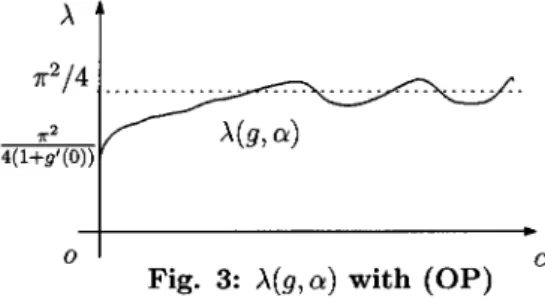
(3) 149. (A.1) g(u)\in C^{1}(\mathbb{R}) and u+g(u)>0 for (A.2) g(u+2 $\pi$)=g(u) for. u>0.. u\in \mathbb{R}.. Then we know from [15] that there exists a unique solution pair ( $\lambda$, u_{ $\alpha$}) of (1.1)-(1.3) with $\alpha$=\Vert u_{ $\alpha$}\Vert_{\infty} for any given. $\alpha$>0. under the condition (A. 1). Besides,. as $\lambda$( $\alpha$) . Moreover, $\lambda$( $\alpha$) is a continuous function of. write $\lambda$= $\lambda$(g, $\alpha$) , since. $\lambda$. $\alpha$>0 .. $\lambda$. is parameterized by. $\alpha$. Then it is convenient for us to. also depends on g . We note that the Fourier series of g converges. uniformly to g . under the conditions (A.1) and (A.2). Now, we introduce the notion of (OP). (OP) $\lambda$(g, $\alpha$)\rightarrow$\pi$^{2}/4 as for. $\alpha$\rightarrow\infty. , and it intersects the line $\lambda$=$\pi$^{2}/4 infinitely many times. $\alpha$\gg 1.. Fig. 3: $\lambda$(g, $\alpha$) with (OP). Since g(u) is bounded in \mathbb{R} by (A.2), it is clear that $\lambda$(g, $\alpha$)\rightar ow$\pi$^{2}/4 as. $\alpha$\rightarrow\infty. . Therefore,. the essential point is to find the condition whether $\lambda$(g, $\alpha$) intersects the line. infinitely many times for. $\alpha$\gg 1 .. On the other hand, if g(u). =. By Theorem 1.1, if. $\lambda$. =. $\pi$^{2}/4. g(u)=\displaystyle \frac{1}{2}\sin^{2n+1}(u) , then (OP) holds.. \displaystyle \frac{1}{2}\sin^{2n}(u) , then (OP) does not hold.. The purpose here is. to find a simple condition, from which we understand whether $\lambda$(g, \mathrm{a}) satisfies (OP) or not immediately. Now we state our main results.. Theorem 2.1 ([20]). Assume that g(u) satisfies (A.1)-(A.2) . Then as. $\lambda$(g, $\alpha$)=\displaystyle\frac{$\pi$^{2}{4}-\frac{$\pi$a_{0}{2$\alpha$}-\frac{1}{$\alpha$}\sqrt{\frac{$\pi$}{2$\alpha$}\sum_{n=1}^{\infty}\frac{ _{$\eta$}{n^{3/2}+O($\alpha$^{-2}). ,. $\alpha$\rightarrow\infty,. (2.1). where. a_{0}:=\displaystyle\frac{1}{$\pi$}\int_{-$\pi$}^{$\pi$}g($\theta$)d$\theta$ , ら \displaystyle \int_{- $\pi$}^{ $\pi$}g'( $\theta$)\cos(n( $\theta$- $\alpha$)+\frac{3}{4} $\pi$)d $\theta$, :=. (2.2). (n\in \mathrm{N}) .. (2.3).

(4) 150. As a corollary of Theorem 2.1, we get an interesting result for the asymptotic behavior of. $\lambda$(g, $\alpha$) .. Corollary 2.2 ([20]). Assume that g(u) satisfies (A.1)-(A.2) . If a_{0}\neq 0 , then $\lambda$(g, $\alpha$) does not satisfy (OP) .. By Corollary 2.2, we understand immediately the reason that, in the case of g(u). =. \displaystyle \frac{1}{2}\sin^{2n+1}(u) , (OP) holds, and in the case of g(u)=\displaystyle \frac{1}{2}\sin^{2n}(u) , (OP) does not hold.. The method to study the local behavior of $\lambda$(g, $\alpha$) has been already obtained in [17,. 18], because the time‐map method and Taylor expansion work very well to study the local structure of. $\lambda$(g, $\alpha$) .. Theorem 2.3 ([20]). Assume (A.1)-(A.2) . Furthermore, assume that g\in C^{2} near u=0. (i) Assume that g(0)\neq 0 . Then as $\alpha$\rightarrow 0,. $\lambda$(g, $\alpha$) = \displaystyle \frac{2 $\alpha$}{g(0)}\{1+A_{1} $\alpha$+A_{2}$\alpha$^{2}+o($\alpha$^{2})\} ,. (2.4). where. A_{1}=-\displaystyle \frac{5}{6g(0)}(1+g'(0) , A_{2}=\frac{32}{45}\frac{(1+g'(0) ^{2} {g(0)^{2} -\frac{11}{30}\frac{g' (0)}{g(0)} .. (2.5). (ii) Assume that g(0)=0 and g'(0)>-1 . Then as $\alpha$\rightarrow 0,. $\lambda$(g, $\alpha$) = \displaystyle \frac{1}{1+g'(0)}(\frac{$\pi$^{2} {4}-\frac{ $\pi$ g'(0)}{3(1+g(0) } $\alpha$+o( $\alpha$) . 3. Global behavior of. (2.6). $\lambda$(g, $\alpha$). The proof of Theorem 2.1 is given by the combination of time‐map method, Fourier expansion. and the asymptotic formulas for some special functions. The proof is given by several steps. In this section, let. $\alpha$\gg 1 .. For simphcity, we write $\lambda$= $\lambda$(g, $\alpha$) . Moreover, we denote by C. the various positive constants independent of. $\alpha$. . Let. G(u) :=\displaystyle \int_{0}^{u}g(s)ds . We know that if. (3.1). (u_{ $\alpha$}, $\lambda$)\in C^{2}(\overline{I})\times \mathbb{R}_{+} satisfies (1.1)-(1.3) , then the following properties hold. u_{ $\alpha$}(t)=u_{ $\alpha$}(-t) , 0\leq t\leq 1 ,. (3.2). u_{ $\alpha$}(0)=\displaystyle \max_{-1\leq t\leq 1}u_{ $\alpha$}(t)= $\alpha$ ,. (3.3). u_{ $\alpha$}'(t)>0, -1<t<0 .. (3.4).

(5) 151. Step 1. The well known time‐map (3.7) below is constructed as follows. By (1.1),. \{u_{ $\alpha$}''(t)+ $\lambda$(u_{ $\alpha$}(t)+g(u_{ $\alpha$}(t)))\}u_{ $\alpha$}'(t)=0. By this and putting. t=0 ,. we have. \displaystyle \frac{1}{2}u_{ $\alpha$}'(t)^{2}+ $\lambda$(\frac{1}{2}u_{ $\alpha$}(t)^{2}+G(u_{ $\alpha$}(t). =. constant. By this and (3.4), for −I \leq t\leq 0 , we have. = $\lambda$(\displaystyle \frac{1}{2}$\alpha$^{2}+G( $\alpha$). .. u_{ $\alpha$}'(t)=\sqrt{ $\lambda$}\sqrt{$\alpha$^{2}-u_{ $\alpha$}(t)^{2}+2(G( $\alpha$)-G(u_{ $\alpha$}(t)))} . It is clear from (A.2) that |g(u)| \leq C for. u\in \mathbb{R} .. (3.5). Then for 0\leq s\leq 1,. |\displaystyle\frac{G($\alpha$)-G($\alpha$s)}{$\alpha$^{2}(1-s^{2})|=\frac{\int_{$\alpha$s}^{$\alpha$}g(t)dt}{$\alpha$^{2}(1-s^{2})|\leq\frac{C$\alpha$(1-s)}{$\alpha$^{2}(1-s^{2})\leqC$\alpha$^{-1} .. By (3.5), (3.6), putting. s. (3.6). :=u_{ $\alpha$}(t)/ $\alpha$ and Taylor expansion, we have. \displaystyle \sqrt{ $\lambda$} = \int_{-1}^{0}\frac{u_{ $\alpha$}'(t)}{\sqrt{$\alpha$^{2}-u_{ $\alpha$}(t)^{2}+2(G( $\alpha$)-G(u_{ $\alpha$}(t) } dt = \displaystyle \int_{0}^{1}\frac{1}{\sqrt{1-s^{2}+2(G( $\alpha$)-G( $\alpha$ s) /$\alpha$^{2} ds = \displaystyle \int_{0}^{1}\frac{1 }{\sqrt{1-s^{2} \sqrt{1+2(G( $\alpha$)-G( $\alpha$ s) /($\alpha$^{2}(1-s^{2}) } ds. (3.7). = \displaystyle \int_{0}^{1}\frac{1}{\sqrt{1-s^{2} \{1-\frac{G( $\alpha$)-G( $\alpha$ s)}{$\alpha$^{2}(1-s^{2}) +O($\alpha$^{-2})\}ds. := \displaystyle \frac{ $\pi$}{2}-\frac{1}{$\alpha$^{2} K( $\alpha$)+O($\alpha$^{-2}). .. Here,. K( $\alpha$) :=\displaystyle \int_{0}^{1}\frac{G( $\alpha$)-G( $\alpha$ s)}{(1-s^{2})^{3/2} ds .. (3.8). Step 2. We calculate K( $\alpha$) by the asymptotic formulas for several special functions as $\alpha$\rightarrow\infty. . We know that under the conditions (\mathrm{A}.1)-(\mathrm{A}.2) ,. g(x) holds for. x\in \mathbb{R}. =. \displaystyle \frac{1}{2}a_{0}+\sum_{n=1}^{\infty}a_{n}\cos nx+\sum_{n=1}^{\infty}b_{n}\sin. and the right hand side of (3.9) converges to g(x) umiformly on. a_{n} = \displaystyle \frac{1}{ $\pi$}\int_{- $\pi$}^{ $\pi$}g( $\theta$)\cos n $\theta$ d $\theta$=-\frac{1}{n $\pi$}\int_{- $\pi$}^{ $\pi$}g'( $\theta$)\sin n $\theta$ d $\theta$ := -\tilde{a}_{n}\underline{1} (n\in \mathbb{N}_{0}) n. .. \mathbb{R} .. Here,. (3.10). ,. b_{n} = \displaystyle \frac{1}{ $\pi$}\int_{- $\pi$}^{ $\pi$}g( $\theta$)\sin n $\theta$ d $\theta$=\frac{1}{n $\pi$}\int_{- $\pi$}^{ $\pi$}g'( $\theta$)\cos n $\theta$ d $\theta$ := \displaystyle \frac{1}{n}\tilde{b}_{n} (n\in \mathrm{N}). (3.9). nx. (3.11).

(6) 152. Step 3.. Lemma 3.1 ([20]). As. $\alpha$\rightarrow\infty,. K($\alpha$)=\displaystyle\frac{1}{2}a_{0}$\alpha$+\frac{1}{$\pi$}\sqrt{\frac{$\pi\alpha$}{2} \sum_{n=1}^{\infty}\frac{ _{n} {n^{3/2} +O($\alpha$^{-1/2}) Proof. We put. \mathcal{S}=\sin $\theta$. .. (3.12). in (3.8). Then we obtain. K( $\alpha$)= $\alpha$\displaystyle \int_{0}^{ $\pi$/2}g( $\alpha$\sin $\theta$)\sin $\theta$ d $\theta$ . We use here the integration by parts and l’Hôpital’s rule. For. (3.13) n=\mathbb{N} ,. let. U_{n} := \displaystyle \int_{0}^{ $\pi$/2}\cos(n $\alpha$\sin $\theta$)\sin $\theta$ d $\theta$ , V_{n} := \displaystyle \int_{0}^{ $\pi$/2}\sin(n $\alpha$\sin $\theta$)\sin $\theta$ d $\theta$ .. (3.14) (3.15). By (3.13)-(3.15) ,. K( $\alpha$) = $\alpha$\displaystyle \int_{0}^{ $\pi$/2}g( $\alpha$\sin $\theta$)\sin $\theta$ d $\theta$. (3.16). = $\alpha$\displaystyle\int_{0}^{$\pi$/2}\{ frac{1}{2}a_{0}+\sum_{n=1}^{\infty}a_{n}\cos(n$\alpha$\sin$\theta$) +\displaystyle\sum_{n=1}^{\infty}b_{n}\sin( $\alpha$\sin$\theta$)\} sin$\theta$d$\theta$ = $\alpha$\displaystyle\{ frac{1}{2}a_{0}+\sum_{n=1}^{\infty}a_{n}\int_{0}^{$\pi$/2}\cos(n$\alpha$\sin$\theta$)\sin$\theta$d$\theta$ +\displaystyle\sum_{n=1}^{\infty}b_{n}\int_{0}^{$\pi$/2}\sin( $\alpha$\sin$\theta$)\sin$\theta$d$\theta$\} = $\alpha$\displaystyle\{ frac{1}{2}a_{0}-\sum_{n=1}^{\infty}\frac{1}{n}\tilde{a}_{$\eta$}U_{n}+\sum_{n=1}^{\infty}\frac{1}{n}\tilde{b}_{n}V_{n}\.. Put $\theta$= $\pi$/2- $\phi$ in (3.22). Then by (3.9)-(3.12) , (3.14), (3.15) and [9, p.425], we obtain. U_{n} = \displaystyle \int_{0}^{ $\pi$/2}\cos(n $\alpha$\cos $\phi$)\cos $\phi$ d $\phi$. = \displaystyle \frac{ $\pi$}{4}(\mathrm{E}_{1}(n $\alpha$)-\mathrm{E}_{-1}(n $\alpha$) = \displaystyle \frac{ $\pi$}{4}(-Y_{1}(n $\alpha$)+Y_{-1}(n $\alpha$)+O((n $\alpha$)^{-2}). = \displaystyle \frac{ $\pi$}{4}(-\sqrt{\frac{2}{n $\pi \alpha$} \sin(n $\alpha$-\frac{3}{4} $\pi$) +\sqrt{\frac{2}{n $\pi \alpha$} \sin(n $\alpha$+\frac{1}{4} $\pi$). (3.17).

(7) 153. +O((n $\alpha$)^{-3/2}). = -\displaystyle \sqrt{\frac{ $\pi$}{2n $\alpha$} \sin(n $\alpha$-\frac{3}{4} $\pi$)+O( n $\alpha$)^{-3/2}). .. Here, \mathrm{E}_{ $\nu$}(z) are Weber functions and Y_{ $\nu$}(z) are Neumann functions. Moreover,. V_{n} = \displaystyle \int_{0}^{ $\pi$/2}\sin(n $\alpha$\cos $\phi$)\cos $\phi$ d $\phi$. (3.18). = \displaystyle \frac{ $\pi$}{4}\{\mathrm{J}_{1}(n $\alpha$)-\mathrm{J}_{-1}(n $\alpha$)\} = \displaystyle \frac{ $\pi$}{4}\{J_{1}(n $\alpha$)-J_{-1}(n $\alpha$)\}. =\displaystyle\frac{$\pi$}{4}\{ sqrt{\frac{2}{n$\pi\alpha$} \cos(n$\alpha$-\frac{3}{4}$\pi$)-\sqrt{\frac{2}{n$\pi\alpha$} \cos(n$\alpha$+\frac{1}{4}$\pi$)\} +O((n $\alpha$)^{-3/2}). = \displaystyle \sqrt{\frac{ $\pi$}{2n $\alpha$} \cos(n $\alpha$-\frac{3}{4} $\pi$)+O( n $\alpha$)^{-3/2}). .. Here, \mathrm{J}_{ $\nu$}(z) are Anger functions and J_{ $\nu$}(z) are Bessel functions) By (3.14)-(3.18) , we obtain. K($\alpha$)= $\alpha$\displaystyle\{ frac{1}{2}a_{0}+\sqrt{\frac{$\pi$}{2$\alpha$} \sum_{n=1}^{\infty}(\tilde{a}_{n}\sin( $\alpha$-\frac{3}{4}$\pi$). +\displaystyle \tilde{b}_{n}\cos(n $\alpha$-\frac{3}{4} $\pi$) \frac{1}{n^{3/2} \}. +O($\alpha$^{-1/2}\displaystyle\sum_{n=1}^{\infty}\frac{1}{n^{5/2} ) = $\alpha$\displaystyle\{ frac{1}{2}a_{0}+\frac{1}{$\pi$}\sqrt{\frac{$\pi$}{2$\alpha$}\sum_{n=1}^{\infty}\frac{ _{m}{n^{3/2}\}+O($\alpha$^{-1/2}). .. Thus the proof is complete. 1. By (3.7) and Lemma 3.1, we obtain Theorem 2.1. 1 We introduce the Special functions and their asymptotic behavior here. For z\gg 1 , we. have (cf. [9, p. 929, p. 958]). J_{1}(z) = \displaystyle \sqrt{\frac{2}{ $\pi$ z} \{[1+R_{1}]\cos(z-\frac{3}{4} $\pi$) ‐. [\displaystyle\frac{1}{2z}\frac{$\Gam a$(\frac{5}{2}){$\Gam a$(\frac{1}{2})+R_{2}]\sin(z-\frac{3}{4}$\pi$)\}. J_{-1}(z) = \displaystyle \sqrt{\frac{2}{ $\pi$ z} \{[1+R_{1}]\cos(z+\frac{1}{4} $\pi$). ,. (3.19).

(8) 154. [\displayst le\frac{\mathrm{I}{2z}\frac{\mathrm{r}(\frac{5}2)}{$\Gam a$(\frac{1}2)}+R_{2}]\sin(z+\frac{1}4 $\pi$)\}. ,. (3.20). +[\displaystyle\frac{1}{2z}\frac{$\Gam a$(\frac{5}{2}){$\Gam a$(\frac{1}{2})+R_{2}]\cos(z-\frac{3}{4}$\pi$)\}. ,. (3.21). +[\displaystyle\frac{1}{2z}\frac{$\Gam a$(\frac{5}{2}){$\Gam a$(\frac{1}{2})+R_{2}]\cos(z+\frac{1}{4}$\pi$)\}. ,. (3.22). ‐. Y_{1}(z) = \displaystyle \sqrt{\frac{2}{ $\pi$ z} \{[1+R_{1}]\sin(z-\frac{3}{4} $\pi$). Y_{-1}(z) = \displaystyle \sqrt{\frac{2}{ $\pi$ z} \{[1+R_{1}]\sin(z+\frac{1}{4} $\pi$) where. |R_{1}|< \displaystyle\frac{$\Gam a$(\frac{7}{2}){8$\Gam a$(-\frac{1}{2})z^{2}|, R_{2}|<|\frac{$\Gam a$(\frac{9}{2}){48$\Gam a$(-\frac{3}{2})z^{3}|. ,. \mathrm{J}_{\pm 1}(z) = J_{\pm 1}(z) , \mathrm{E}_{\pm 1}(z). 4. =. -Y\pm 1(z) 干. (3.23). (3.24). \displaystyle \frac{2}{ $\pi$ z^{2} +O(z^{-4}) .. (3.25). Special case. Finally, we are interested in the case g(u) =\sin\sqrt{u} . In this case, the equation (1.1)-(1.3). has been proposed in Cheng [5] as a model problem which has arbitrary many solutions near $\lambda$=$\pi$^{2}/4. Theorem 4.0.([5]) Let g_{1}(u)=\sin\sqrt{u} (u\geq 0) . Then for any integer r\geq 1 , there is such that if $\lambda$\in($\lambda$_{1}- $\delta,\ \lambda$_{1}+ $\delta$) , then (1.1)-(1.3) has at least. r. $\delta$>0. distinct solutions.. Theorem 4.0 gives us the imformation about the solution set of (1.1)-(1.3) , and we expect. that $\lambda$(g_{1}, $\alpha$) satisfies (OP). The purpose here is to prove the expectation above is valid.. Theorem 4.1 ([21]). Let g(u)=g_{1}(u)=\sin\sqrt{u} . Then as. $\alpha$\rightarrow\infty,. $\lambda$(g_{1}, $\alpha$) = \displaystyle \frac{$\pi$^{2} {4}-$\pi$^{3/2}$\alpha$^{-5/4}\cos(\sqrt{ $\alpha$}-\frac{3}{4} $\pi$)+o($\alpha$^{-5/4}) . We next give the asymptotic behavor of $\lambda$(g_{1}, $\alpha$) as. (4.1). $\alpha$\rightarrow 0.. Theorem 4.2 ([21]). Let g(u)=g_{1}(u)=\sin\sqrt{u}. (i) As. $\alpha$\rightarrow 0 ,. the following asymptotic formula for $\lambda$(g_{1}, $\alpha$) holds:. $\lambda$(g_{1}, $\alpha$) = \displaystyle \frac{3}{4}C_{1}^{2}\sqrt{ $\alpha$}+\frac{3}{2}C_{1}C_{2} $\alpha$+O($\alpha$^{3/2}) ,. (4.2).

(9) 155. where. C_{1}:=\displaystyle \int_{0}^{1}\frac{1}{\sqrt{1-s^{3/2} }ds, C_{2}:=-\frac{3}{8}\int_{0}^{1}\frac{1-s^{2} {\sqrt{1-s^{3/2} }ds . (ii) Let. v_{0}. (4.3). be a unique classical solution of the following equation. -v_{0}' (t) = \displaystyle \frac{3}{4}C_{1}^{2}\sqrt{v_{0}(t)}, t\in I ,. (4.4). v_{0}(t) > 0, t\in I ,. (4.5). v_{0}(-1) = v_{0}(1)=0 .. (4.6). Furthermore, let v_{ $\alpha$}(t) :=u_{ $\alpha$}(t)/ $\alpha$ . Then. v_{ $\alpha$}\rightarrow v_{0}. in C^{2}(I) as. $\alpha$\rightarrow 0.. The proofs also depend on time‐map method.. References [1] A. Ambrosetti, H. Brezis, G. Cerami, Combined effects of concave and convex nonlin‐ earities in some elliptic problems, J. Funct. Anal., 122 (1994), 519‐543. [2] S. Cano‐Casanova and J. López‐Gómez, Existence, uniqueness and blow‐up rate of large solutions for a canonical class of one‐dimensional problems on the half‐line, J.. Differential Equations, 244 (2008), 3180‐3203. [3] S. Cano‐Casanova, J. López‐Gómez, Blow‐up rates ofradially symmetric large solutions, J. Math. Anal. Appl., 352 (2009), 166‐174.. [4] Shanshan Chen, Junping Shi and Junjie Wei, Bifurcation analysis of the Gierer‐ Meinhardt system with a saturation in the activator production, Appl. Anal., 93 (2014), 1115‐1134.. [5] Y.J. Cheng, On an open problem of Ambrosetti, Brezis and Cerami, Differential Integral Equations, 15 (2002), 1025‐1044. [6] R. Chiappinelli, On spectral asymptotics and bifurcation for elliptic operators with odd superlinear term, Nonlinear Anal., 13 (1989), 871‐878. [7] J. M. Fraile, J. López‐Gómez and J. Sabina de Lis, On the global structure of the set of positive solutions of some semilinear elliptic boundary value problems, J. Differential. Equations, 123 (1995), 180‐212..

(10) 156. [8] A. Galstian, P. Korman and Y. Li, On the oscillations of the solution curve for a class of semilinear equations, J. Math. Anal. Appl., 321 (2006), 576‐588. [9] I. S. Gradshteyn and I. M. Ryzhik, Table of integraJs, series, and products. Translated from the Russian. Translation edited and with a preface by Daniel Zwillinger and Victor. Moll. Eighth edition. Elsevier/Academic Press, Amsterdam, 2015. [10] P. Korman and Y. Li, Exact multiplicity of positive solutions for concave‐convex and convex‐concave nonlinearities, J. Differential Equations, 257 (2014), 3730‐3737.. [11] P. Korman and Y. Li, Computing the location and the direction of bifurcation for sign changing solutions, Differ. Equ. Appl., 2 (2010), 1‐13. [12] P. Korman and Y. Li, Infinitely many solutions at a resonance, Electron. J. Differ. Equ. Conf. 05, 105‐111.. [13] P. Korman, An oscillatory bifurcation from infinity, and from zero,. NoDEA. Nonlinear. Differential Equations Appl., 15 (2008), 335‐345.. [14] P. Korman, Global solution curves for semilinear elliptic equations, World Scientific Publishing Co. Pte. Ltd., Hackensack, NJ, (2012). [15] T. Laetsch, The number of solutions of a nonlinear two point boundary value problem, Indiana Univ. Math. J., 201970/19711‐13. [16] T. Shibata, New method for computing the local behavior of L_{q} ‐bifurcation curve for logistic equations, Int. J. Math. Anal., (Ruse) 7 (2013) no. 29‐32, 1531‐1541.. [17] T. Shibata, \mathrm{S} ‐shaped bifurcation curves for nonlinear two‐parameter problems, Nonlin‐ ear Anal., 95 (2014), 796‐808.. [18] T. Shibata, Asymptotic length of bifurcation curves related to inverse bifurcation prob‐ lems, J. Math. Anal. Appl., 438 (2016), 629‐642. [19] T. Shibata, Oscillatory bifurcation for semilinear ordinary differential equations, Elec‐ tron. J. Qual. Theory Differ. Equ. 2016, No. 44, 1‐13.. [20] T. Shibata, Global behavior of bifurcation curves for the nonlinear eigenvalue problems with periodic nonlinear terms, to appear.. [21] T. Shibata, Global and local structures of oscillatory bifurcation curves with application to inverse bifurcation problem, to appear..

(11)