Faster Algorithms for Computer Vision (The advances and applications of optimization method)

Faster Algorithms

for

Computer

Vision

Toshiyuki

Masaki

and Takahito

Kuno

Graduate School of Systems and Information Engineering,

University of Tsukuba, Ibaraki 305-8573, Japan

Abstract

In this paper, we make amodification to Karl and Hartley‘s formulation

ofproblems in computervision [3, 4], and show the resulting norm

min-imization problemcan be solvedby solving a sequence of LP problems.

We also propose an approximation of the norm minimization problem,

which reduces to one LP or SOCP problem.

Key words: Computer vision, multiple view geometry, linear

program-ming, second-order cone programming.

1.

Introduction

In recent years, problems dealt with in computer vision

are

larger in size and

require much

more

computational time to solve than before. For example,

while the traditional triangulation problem has only three variables, the

num-ber of variables in the latest structure-and-motion problem amounts to several

hundreds in

some cases.

Thus, there is a great need for faster algorithms for

large scale problems in the

area

of computer vision. In response to this, Karl

and Hartley [3, 4] developed a framework for solving geometric problems, such

as

triangulation, camera-resectioning, homography-estimation and

structure-and-motion. In their framework, those problems are formulated into an $L_{\infty}$

norm

minimization problem and solved by solving a sequence of second-order

cone

programming (SOCP) problems.

In this paper, we show that, if Karl and Hartley‘s formulation is slightly

modified, the norm $1ni_{I}iiInizati_{oI}i$ problem can be solved by solving a sequence

of linear programming (LP) problems. In addition,

we

propose

an

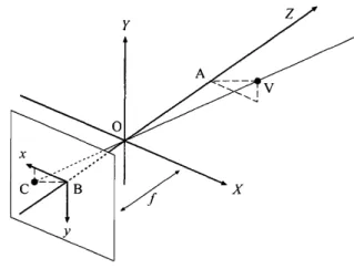
Figure 1: Geometry of a pinhole camera.

problem. Lastly, we report

some

numerical results, which demonstrate the

superiority of our approach to Karl and Hartley‘s in both efficiency and

accu-racy.

2.

Problems

in

computer

vision

In this section, we first take triangulation

as a

typical example and illustrate

how it can be formulated into an optimization problem. We also show that

many other problems in computer vision take the

same

form. Essential to

those formulations is the pinhole camem model.

Pinhole

camera

model: The pinhole

camera

model describes the

relation-ship between the coordinates of

a

$3D$ point and its projection onto the image

plane of

an

ideal pinhole camera, where the

camera

aperture is a pinhole and

no

lenses

are

used to focus light. The geometry related to the mapping of

a

pinhole

camera

is illustrated in Figure 1. Let

us

denote the object point by

$V=(X, Y, Z)^{T}$ _{in the}$3D$ coordinate system withits originat the

camera

aper-ture O. Light emanating from V passes through $O$ and projects

an

inverted

image $v=(x, y)^{T}$

on

the _{image plane, which is parallel to the} X-Y _plane and

located at the focal length $f(>0)$ from $O$ in the negative direction of the

$Z$ axis. Let A _{$=(0,0, Z)^{T},$} $B=(0,0, -f)^{T}$ and $C=(x, y, -f)^{T}$. Since the

Figure 2: Thriangulation using two

cameras.

or

equivalently

$\{\begin{array}{l}xy1\end{array}\}=\frac{f}{Z}\{\begin{array}{l}XYZ/f\end{array}\}$

in homogeneous coordinates. It should be also noted that the image $v$ is

invariant under scaling ofV. We denote this by

$\{\begin{array}{l}xy1\end{array}\}\sim\{\begin{array}{l}XYZ/f\end{array}\}=\{\begin{array}{llll}1 0 0 00 1 0 00 0 1/f 0\end{array}\}\{\begin{array}{l}XYZ1\end{array}\}$ , (1)

and say that $(x, y, 1)^{T}$ is equivalent,

or

proportional, to $(X, Y, Z/f)^{T}$. The $3\cross 4$

matrix in (1) is called the

camem

matrix.

Triangulation: Triangulation (or reconstruction) is the process of

deter-mining the $3D$ coordinates of the object V, given its projection onto two, or

more, images captured by pinhole

cameras.

In theory, the triangulation

prob-lem is quite trivial. Each image $v$ of V corresponds to

a

half-line in the $3D$

space such that all points on the line

are

projected to $v$. Therefore, V must

lie

on

the intersection of those lines, and

we

must be able to calculate its

co-ordinates analytically from a pair of different images. In practice, however,

various types of noise, such

as

geometric noise from lens distortion

or

interest

point detection error, lead to inaccuracies in the measured image coordinates.

As a result, lines associated with different images ofV do not always intersect

Suppose that is in

an

arbitrary coordinate system, and

that there

are

$M$ images $v_{i}=(x_{i}, y_{i})^{T}$ ofV capturedby

cameras

$i=1,$

$\ldots,$$M$.

Let

us

denote the ith

camera

matrix by

$Q_{i}=\{\begin{array}{llll}1 0 0 00 1 0 00 0 1/f_{i} 0\end{array}\}$ ,

where $f_{i}(>0)$ is the focal length of

camera

$i$. Note that V is denoted

as

$B_{n}V+t_{i}$ for

some

rotation matrix $B_{\eta}$ and

a

translation vector $t_{i}$ in the $3D$

coordinate system with the origin at the focal point $O_{i}$ of

camera

$i$. Hence,

from (1),

we

have

$\{\begin{array}{l}v_{i}1\end{array}\}\sim Q_{i}\{\begin{array}{ll}R_{n} t_{i}O 1\end{array}\}\{\begin{array}{l}V1\end{array}\}$ , $i=1,$

$\ldots,$$M$.

Let

$P_{i}=\{\begin{array}{l}p_{i}^{1}p_{i}^{2}p_{i}^{3}\end{array}\}=Q_{i}\{\begin{array}{ll}R_{i} t_{i}O 1\end{array}\}$ ,

which is referred to

as

the normalized

camem

matrix,

or

simply

as

the

camem

matrix. The coordinates of the image $v_{i}=(x_{i}, y_{i})^{T}$ is then given

as

$x_{i}= \frac{p_{i}^{1}U}{p_{i}^{3}U}$, $y_{i}= \frac{p_{i}^{2}U}{p_{i}^{3}U}$,

where $U=(V^{T}, 1)^{T}$, if there is no noise. As mentioned above, however, this is

not the casein practice, and we need to determine the coordinates $(X, Y, Z)$ of

V

so

as to minimize the $2D$ residual ermr, which is defined as follows in terms

of $L_{p}$

norm:

$\gamma_{i}=\Vert\frac{p_{i}^{1}U}{p_{i}^{3}U}-x_{i},\frac{p_{i}^{2}U}{p_{i}^{3}U}-y_{i}\Vert_{p}$ , $i=1,$

$\ldots,$ $M$.

If

we

measure

the magnitude of $\gamma=(\gamma_{1}, \ldots, \gamma_{M})^{T}$ in $L_{q}$ norm, then

trian-gulation reduces to an optimization problem with $(X, Y, Z)$_, the first three

components of$U$,

as

the variables:

minimize $\Vert\gamma\Vert_{q}$

subject to $\Vert\frac{p_{i}^{1}U}{p_{i}^{3}U}-x_{i},$$\frac{p_{i}^{2}U}{p_{i}^{3}U}-y_{i}\Vert_{p}=\gamma_{i}$, $i=1,$ _$\ldots$ ,M.

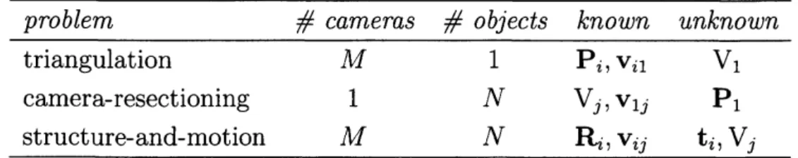
Table 1: Known and unknown parameters of computer vision problems.

$\frac{problem\neq camems\neq objectsknownunknown}{triangu1ationM1P_{i},v_{i1}V_{1}}$

camera-resectioning 1 $N$ _{$V_{j},$ $v_{1j}$} $P_{1}$

structure-and-motion $M$ $N$ $B_{n},$$v_{ij}$ $t_{i},$$V_{j}$

Other problems: Many other computer vision problems

can

also be

for-mulated into optimization problems similar to (2) except that the number of

objects is usually

more

than

one.

Suppose $N$ points $V_{j}=(X_{j}, Y_{j}, Z_{j})^{T},$ $j=1,$

$\ldots,$ $M$, are given in the $3D$

space. Let $v_{ij}=(x_{ij}, y_{ij})^{T}$ denote the image of$V_{j}$ captured by

camera

$i$. Also

let

$\gamma_{ij}=\Vert\frac{p_{i}^{1}U_{j}}{p_{i}^{3}U_{j}}-x_{ij},$$\frac{p_{i}^{2}U_{j}}{p_{i}^{3}U_{j}}-y_{ij}\Vert_{p}$, $i=1,$

$\ldots,$$M;j=1,$ $\ldots N$,

where $U_{j}=(V_{j}^{T}, 1)^{T}$. In this case, the problem is written

as

follows

minimize $\Vert\gamma\Vert_{q}$

subject to $\Vert\frac{p_{i}^{1}U_{j}}{p_{i}^{3}U_{j}}-x_{ij},$ $\frac{p_{i}^{2}U_{j}}{p_{i}^{3}U_{j}}-y_{ij}\Vert_{p}=\gamma_{ij}$, $\{\begin{array}{ll}i=1, \ldots, M (3)j=1, \ldots N, \end{array}$

where $\gamma=(\gamma_{11}, \ldots, \gamma_{MN})^{T}$. This

seems

a straightforward extension of (1),

but describes various types ofproblems in computer vision depending

on

what

parameters

are

known

or

unknown. Table 1 shows three major examples; e.g.,

the number of variables amounts to$3(M+N)$ in (3) associated with

a

structure-and-motion problem while that is only three in the

case

oftriangulation.

3.

Solution

approaches

In [4], Kahl and Hartley proposed

a

bisection algorithm to solve (3) with$p=2$

and $q=\infty$. After illustrating their algorithm, we introduce here a practical

approximation approach to (3).

Bisection approach: In the usual applications ofcomputer vision, we may

$\overline{\frac{A1gorithm1Bisectionalgorithmforthecasewherep=2andq=\infty}{Require:aninterva1[\gamma_{\ell},\gamma_{u}]knowntocontaintheoptima1va1uer^{*}and}}$

a

tolerance $\epsilon>0$.

repeat

$\gammaarrow(\gamma_{\ell}+\gamma_{u})/2$;

check if (5) is feasible

or

not, by solving

an

associated SOCP problem;

if (5) is feasible then $\gamma_{u}arrow\gamma$ else $\gamma_{\ell}arrow\gamma$ end if until $\gamma_{u}-\gamma_{l}\leq\epsilon$;

when $p=2$ and $q=\infty$:

minimize $\gamma$

subject to $\Vert p_{i}^{1}U_{j}-x_{ij}p_{i}^{3}U_{j},$ $p_{i}^{2}U_{j}-y_{ij}p_{i}^{3}U_{j}\Vert_{2}\leq\gamma p_{i}^{3}U_{j}$, $\{\begin{array}{l}i=1, \ldots, Mj=1, \ldots N.\end{array}$

(4)

As is shown in Algorithm 1, the bisection algorithm solves (4) by checking

repeatedly if the following system of inequalities is feasible for a fixed $r$ in a

given interval $[\gamma_{\ell}, \gamma_{u}]$:

$\Vert p_{i}^{1}U_{j}-x_{ij}p_{i}^{3}U_{j},$ $p_{i}^{2}U_{j}-y_{ij}p_{i}^{3}U_{j}\Vert_{2}\leq\gamma p_{i}^{3}U_{j},$ $\{\begin{array}{l}i=1, \ldots, Mj=1, \ldots N.\end{array}$ (5)

Since the right-hand-sides turn into constants, the feasibility of (5) can be

checked by solving

an

SOCP problem with (5)

as

constraints.

As

a

natural extension of this Kahl and Hartley’s approach,

we can

ap-ply the bisection algorithm to (3) with another combination of$p$ and $q$. For

example, if we choose$p=1$ and $q=\infty$, then (3) is rewritten as

minimize $\gamma$

subject to $|p_{i}^{1}U_{j}-x_{ij}p_{i}^{3}U_{j}|+|p_{i}^{2}U_{j}-y_{ij}p_{i}^{3}U_{j}|\leq\gamma p_{i}^{3}U_{j}$, $\{\begin{array}{l}i=1, \ldots, Mj=1, \ldots N.\end{array}$

(6)

Note that the inequality

is equivalent to

a

set of inequalities

$-(p_{i}^{1}U_{j}-x_{ij}p_{i}^{3}U_{j})-(p_{i}^{2}U_{j}-y_{ij}p_{i}^{3}U_{j})\leq\gamma p_{i}^{3}U_{j}-(U_{j}-xp^{3}U_{j})+(-y_{ij}p^{3})\leq\gamma p^{3}U_{j}(U_{j}U_{ji}(p^{1}U-xp^{3}U)+(U_{j}p_{i}^{3}U)\leq\gamma p^{3}U_{j}p^{2}-y_{ij}p_{i}^{3})\leq\gamma p^{3}U_{j}$

.

$\}$ (7)

In other words, the constraints of (6) can be thought of

as

linear constraints

once

the value of$\gamma$ is

$fix\epsilon_{\text{ノ}}^{\backslash }(1$. Hence, Algorith11l 1

can

solve (6) by checking the

feasibility of (7) for all $i,j$, instead of (5). This

can

be done by solving

an

LP

problem with (7) for all $i,j$

as

constraints. Similarly,

we

can

solve (3) with

$p=\infty$ and $q=\infty$ using the bisection algorithm.

Approximation approach: The

reason

why (3) cannot be solved directly

as an

SOCP

or

LP problem is that the product oftwo variables appears in the

right-hand-sides of the constraints when (3) is rewritten

as

minimize $\Vert\gamma\Vert_{q}$

subject to $\Vert p_{i}^{1}U_{j}-x_{ij}p_{i}^{3}U_{j},$ $p_{i}^{2}U_{j}-y_{ij}p_{i}^{3}U_{j}\Vert_{p}=\gamma_{ij}p_{i}^{3}U_{j}$, $\{\begin{array}{l}i=1, \ldots, Mj=1, \ldots N.\end{array}$

(8)

Introducing

new

variables $\delta_{ij}$ and letting

$\delta_{ij}=\gamma_{ij}p_{i}^{3}U_{j}$, $i=1,$

$\ldots,$$M;j=1,$ $\ldots,$$N$,

we

have

minimize $\Vert\delta\Vert_{q}$

subject to $\Vert p_{i}^{1}U_{j}-x_{ij}p_{i}^{3}U_{j},$ $p_{i}^{2}U_{j}-y_{ij}p_{i}^{3}U_{j}\Vert_{p}=\delta_{ij}$, $\{\begin{array}{l}i=1, \ldots, Mj=1, \ldots N,\end{array}$

(9)

where $\delta=(\delta_{11}, \ldots, \delta_{MN})^{T}$. It is easy to

see

that (9) reduces to

an

SOCP

problem if $p=2$ and $q=\infty$, and is

an

LP problem if $p=1,$ $\infty$ and _$q=\infty$.

Furthermore, (9)

can

serve as a

good approximation for (8) (and hence (3)).

Proposition 1

_If

the optimal value

_of

(8) vanishes, then any optimal solution

of

(8), together with$\delta=O$, solves (9) to optimality. Conversely,

if

the optimal

value

_of

(9) vanishes, then any optimal solution

_of

(9), together with $\gamma=O$,

Table 2: CPU time (in seconds).

$\frac{p\backslash q\infty 12}{bisection\infty 0.0660.1170.729}$

$\infty$

0.003

0.003

0.075

approximation

1 0.009 0.004 0.080

Table 3: $3D$ residual error (in $L_{2}$ norm).

$\frac{p\backslash q\infty 12}{bisection\infty 0.0170.0180.016}$

$\infty$ 0.036 0.036 0.035

approximation

1 0.014 0.014 0.013

Let

us

discuss the

case

where $q=\infty$ a little

more

closely. Let $(\overline{\gamma}_{ij}, \overline{p_{i}^{3}U_{j}})$

and $(\overline{\delta}_{ij},\overline{p_{i}^{3}U_{j}})\wedge$

denote the values of $(\gamma_{ij}, p_{i}^{3}U_{j})$ for optimal solutions of (8) and

(9), respectively, and define

$\gamma$

へ

$=\delta/p_{k}^{3}U_{l}$, $\overline{\delta}=\overline{\gamma}\overline{p_{r}^{3}U_{s}}$,

where $\overline{\gamma}=\overline{\gamma}_{k\ell}\in\max_{i,j}\{\overline{\gamma}_{ij}\}$ and $\hat{\delta}=\hat{\delta}_{rs}\in\max_{i,j}\{\overline{\delta}_{ij}\}$へ.

Proposition 2 When $q=\infty$, the following relations hold:

$\overline{\gamma}\leq$

へ

$\gamma\leq L\overline{\gamma}$, へ

$\delta\leq\overline{\delta}\leq L\hat{\delta}$,

where $L= \max_{i,j}\{\overline{p_{i}^{3}U_{j}}\}/\min_{i,j}\{\overline{p_{i}^{3}U_{j}}\}$. $\square$

4.

Numerical

results

Lastly,

we

report

some

numerical results obtained with MATLAB (version 7.9,

$R2009b)[5]$.

The problem used

as

a benchmark istriangulation. The number of

cameras

was

fixed at $N=25$, and each

camera

matrix was of the form:

where $z_{i}$ and $\phi_{i}$

are uniform random

numbers

on

the intervals [10.0, 100.0]

and

$[$0.0, $\frac{\pi}{6}]$, respectively, and

$\theta_{i}=\frac{2\pi}{n(i-1)}$

.

Each component ofthe object point V

was

also generated uniformly at random

in the interval $[-5.0,5.0]$

.

_{Associated SOCP and LP} problems

were

solved

using SeDuMi [7] and GLPK[I], respectively. Table 2 summarizes the average

CPU time in seconds taken to solve ten instances for each $p,$$q$. Table 3 shows

the average residual

error

between actualand calculatedvalues of V in$L_{2}$

norm.

These results suggest that

our

approach is superior to Karl and Hartley‘s in

both efficiency and accuracy.

References

[1] GLPK(GNU LinearProgramming Kit) $http.\cdot//www$.gnu.$org/software/glpk/$.

[2] Hartley, R.I. and Sturm, P. , Triangulation In COMPUTER

ANALYSIS

OF IMAGES AND PATTERNS, pages 190-197, 1995.

[3] Kahl, F. , Multiple view geometry and the $L_{\infty}$

-norm.

In Int.

Conf.

Com-puter Vision,pages 1002-1009, Beijing, China,

2005.

[4] Kahl, F. and Hartley, R.I. , Multiple View Geometry Under the $L_{\infty}$

-norm.

In IEEE Tmnsactions on Pattem Analysis and Machine Intelligence, pages

1603-1617, September 2008.

[5] MATLAB $www.mathworks.com/pmducts/matlab/$.

[6] Olsson, C. and Kahl, F. , Generalized Convexity in Multiple View

Ge-ometry. In JOURNAL OF MATHEMATICAL IMA GING AND VISION,

pages 35-51, September 2010.

[7] SeDuMi $http.\cdot//sedumi.ie.lehigh.edu/$.

[8] Seo, Y. and Hartley, R.I. , Sequential $L_{\infty}$ Norm Minimization for

Tri-angulation. In Computer Vision - ACCV 2007, vol. 4844, pages 322-331,