An Approximate Analysis of One-Dimensimensional Unsteady State Heat Conduction: University of the Ryukyus Repository

Title

An Approximate Analysis of One-Dimensimensional Unsteady

_{State Heat Conduction}

Author(s)

Nagata, Takashi

Citation

琉球大学理工学部紀要. 工学篇 = Bulletin of Science &

Engineering Division, University of the Ryukyus.

Engineering(3): 27-36

Issue Date

1970-06

URL

http://hdl.handle.net/20.500.12000/23948

An Approxi mate Anal ysis of One- Oi mensi mensi on al

Unsteady State Heat

Conduction~

Takashi

Nagata·

An approximate solution based on the heat balance integral equation for one-dimensional unsteady state heat flow in a semi-infinite slab and an infinite plate is discussed. The heat balance integral equation similar to K~rman's integral momentum equati61t for the boundary layer flow leads to the simplification of analysis on the

heat conduction problemi:

Solutions for the temperature distribution and the heat transfer rate fit well with the exact solutions of the heat energy equation, or the diffusion equation.

1. Introduction

Heat conduction problems especially in engineering fields have been actively improved so far with development of applied mathematic~}. In many cases mathematical approach to the diffusioo equation gives series of solutions, and the calculation of heat flux and temperature variation with time at an arbitrary point is troublesome work in practice. Therefore, it is meamngful to find out and develop an algorithm for the approximate solutions.

This paper presents an approximate solution for one-dimensional unsteady state heat conduction problems on a semi-infinite slab and an infinite plate. The main idea discussed in this paper is based on the application of Karnuln's integral momentum theory on the boundary layer flow to the heat conduction system.

-Temperature profiles and heat flux in the body obtained by this approximate ap-proach are discussed in comparison with the exact solutions of the diffusion equation, and furthermore, the method is extended to the infinite plate problem to obtain a tran-sient period and a trantran-sient temperature distribution.

27

Nomenclature a.b.c. : Variable coefficients Cp: Specific heat at constant

pressure

F.:

Fourier modulus G : Mass flux vector h : Specific enthalpy k : Thermal conductivity L: Thickness of a plate

n :

Outward unit normal

vector Subscript

i : Denotes quantity at an initial condition aD : Denotes quantity at the wall surface o : Denotes quantity at x= 0

/) : Denotes quantity at x= /)

ci.:

Heat generation rate q;: Heat flux S : Control surface v ; Control volume Ii : Flow velocity a : TherIl)al diffusivity Jl :Specific mass 't' : Time coordinate

o :

Propagating heat wave

~Received Oct. 31, 1969

28 Nagata :An Approximate Analysis of One-Dimensional Unsleady State Heal Conduction

2. Anal ysi5 of the heat energy equati on

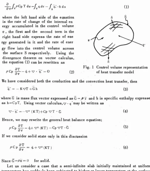
Let us take a control volume as shown in Fig. 1 in the heat transfer system. Con-sidering the conduction and the ~onvectionhe~t transfer at and in the boundary, the application of the conservation law of energy to it leads to the equation,

~

r

pCp T

dv~r

q,.dv - /

q;·n

ds (1)

aT:Jv Jv 5

where the left hand side of the equation is the rate of change of the internal en ergy accumulated in the control volume

v,

the first and the second term in the right hand side express the rate of ene rgy generated in it and the rate of ener gy flow into the centrol volume across

the surface S respectively. Using the divergence theorem on vector calculus, the equation (1) can be rewritten as

v

q...

C a T . -. 0

p p - - q , . + v · q,. = aT:

Fig. 1 Control volume representation of heat transfer model

We have considered both the conduction and the convection heat transfer, then

~'= -KvT+Gh (3)

where G is mass flux vector expressed as G =.P

v

and h is specific enthalpy expressed as h=C pT. Using vector calculus,

v .

q, •may be" written as

v·

q:

~-v' (KT)+Cp vT . G

Hence, we may rewrite the general heat balance equation;

pCp aT

~ti+V'(KT)-CpVT.G

aT:

If

we consider solid state only in this discussion aT

pCPar= ti-+V'(KT)

(5)

SinceG=pli= 0 for solid.

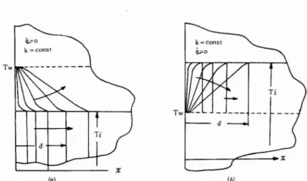
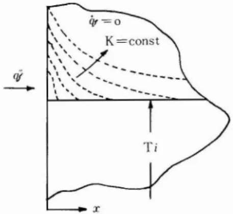
Let us consider a case that a semi-infinite slab initially maintained at uniform temperature has suddeilly been subjected to higher or lower temperature at the surface. The portion influenced by the impressed temperature at its surface will spread itself to the inner part of the slab such a way as shown in Fig. 2. Finally the inside tem-perature will be maintained ;1t the level of the dashed line in the figure. In this simple analysis we see the increasing or decreasing temperature inside it and the thickness influenced will propagate into the slab as a kind of heat wave, and the propagating speed, that is, the rate.oflchange of the thickness could be found as a function of time

Bull. Science & Engifleering Div .• Univ. of the Ryukyus (Engineering) iL.=o k=const Tw Tw x ~

w

Fig. 2 Impressed temperature system of the semi-infinite slab

Purely mathematical approach for this kind of the problem is discussed in a field of the boundary value problems of partial differential equations and the s,olution is expressed as an error function. However, it is possible to attack this problem from a different standpoint by applying the control volume method in the boundary layer flow theory.

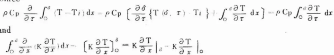
Let /) be the thickness influenced by the propagation of heat wave at some arbitrary time. The mechanics of heat flow in the case is shown in Fig. 3. Integrating the one-dimensional heat equation (6) with respect to the coordinate:l: with considering no heat source in the system,

29 ti=o k=const

T

Tw

I

(Jro I

I

L

:

J

s

-~:__-...,.'---X

Fig. 3 Mechanics of heat flow in the semi-infinite slab

i.0~

(

KaT) dx=

J

°pCp aT dx

oaT'

ax

0

aT'

Expansion of the equation gives

K~

I

-K aaT

I

=pCp

~fa

(T-Ti)dx

~u Nagala :An Approximal<' Allalysis "f Oll"~~ IJillll'lIs;ollal l!II;"'ady Slate lI"al Conduction Since pCp

aa

r

.£"

(T~Ti)dx ~.'

pCp

[~:~T

(0, r). Ti

}!

;;"~;

dx

J

~fJCpfa'i~;'

dr and

1

<$

a

aT

(a

l'

1

iJ =

KaT

I _

al'

I

o d'XiKcrr)dx- K

a-;

0

a-;

,j Ka:;:- 0

This is a heat balance integral equation, the l.eft and the right hand side of the equa-tion represent the net heat flux into the system and the rate of increasing heat energy in the domain respectively.

It

is required to assume a temperature distribution Tk;,r) in order to evaluate the equation (8), that is, once a trial temperature profile with un-known coefficients is assumed, these coefficients are completely determined as func-tions of 0 only by the application of the initial and the boundary conditions as follows;

'I· K -

aT

_a

_x

I

_x=o --- for a given heat flux system

T(<) r) - Tu' _{...---- for an impressed temperature at the face system} T (0. r) . Ti. l' (ee, r) = finite

After obtaining the trial temperature profi

Ie,

integration of the equation (8) can be evaluated and the propagating heat wave 0 is given as a function of r.

Trial temperature profiles, propagating heat wave and heat transfer rate based on this analysis for both the impressed temperature system and the given heat flux system and the given heat flux system are summarized in table 1 and table 2.

Table 1 Comparison of the trial solutions with the exact solution for the impressed temperature system of

the semi-infinite slab. 8(%, -r) ~T (x, -r) -1'W, 8 i=T i-1'W

Temperature distribution Heat flux Heat wave %error in

heat flux Exact solution

o

(x.1') X KOi

o

i = ed( 2[m)

i'=---

Jrra'T

Trial solution (1) O(x.~ 2(

a) - (a /

KOi

0=

J 12ar +2.3% (J j c ( . - - - -- J3«r Trial solution (2) KOi

o

(x,r) ~ 3(L) - 3(L)2+(.!./

0=

j 24ar +8.5% Oi

{)

0

8

q;:~-J

%

aT Trial solution (3)

O(r r)

~

4(2:.)-6(L/+4(L)1- (L/ q;F= K(Ji

a =J

40ar + 12. 2%

(J i

0

{)

8

'0

J 2.50«r

.-Trial solution (4)

(J (x,r)

Sin (.1!.. L) K8i

_{o = J b}

aT -4·4%

71'-Bull. Science &1 Engineering Div., Univ. of the Ryukyus iEngineering) 31

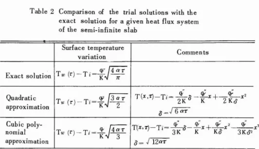
Table 2 Comparison of the trial solutions with the exact solution for a given heat flux system of the semi-infinite slab

Surface temperature

Comments variation

~J!f!

Exact solution T w(r)-Ti=K 7 (

-T( 1') . qf qf

+

qf 2

Quadratic

qrJIV

x -Tl=--a--x - - x

Tu; (r)-Ti=K -Z- ' ZK K Z

Ko

approximation o~.f6(XT Cubic poly-Tw (<)-Ti=

i..J4~r

q;.'

q;.'

qf2

q;

nomial T(x,Tj-Ti= 3K8-j(x+

Ko

x -3KQ2 approximation

₀₌

j

1Zar

3. Di scussi on

The mathematical analysis discussed in the previous secti00 is different from the usual approach to the solutions of the partial differentia1lequations but leads to almost same results compared with the exact soluti00 in the one-dimensional unsteady heat conduction system.

The propagating heat wave cS introduced in this analysis is invariant with the temperature difference between the impressed temperature at the surface and the initial temperature in the solid, but related to the thermal diffusivity a of the materials. Hence, the larger the value of a, the faster will heat diffuse through the material, and also the heat wave propagates thr ough the material in proportion to the square of

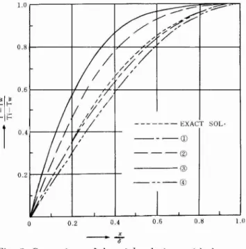
the time coordinate as shown in Fig. 4. Fig. 5 represents the comparison of solu-tions by the present approximate method and by the exact eqation (6) for the impress-ed temperature system. The propagating heat wave and the heat transfer rate for the quadratic expression give a fairly good approximation. The percentage error of heat transfer rate relative to that of the exact solution is 2.3 percentage.

Table 2 represents the comparison of the surface temperature variation with time by the approximate method and by the exact equation (6) for the given heat flux at the face system sh own in Fig. 6. A quadratic or a cubic polynomial approximation gives a satisfactory temperature history at the face comparing with the exact solution.

32 Nagata:An Approximate Analysis of One--Dimensional UnS1l'aJy State Heat ConJuction

v

V

,,,'"

' /

..., ...-

...

, , /

,

, , /

,,

...

"

' ",,-, ' -, / " ,

v

. /

V

_"

"

... ,

"

.-.-

.,V

, / ...

_.-.-

,

/,,,-

,...,,/ ,-""

V'

_V

,, ; , / , _,-"

.

... ,

--

/ ' ; , ; ;,-"

/

.

.-.-(

- - - - ( 1 )

V , / '

, 1 - - - @ « ₂

W

_@ - - - @

I I I II

1.0 5x 10-2x 10--10 - , - 7 '

Fig. 4 Relation between the propagating heat wave 0 and the time7'. The number in circles refers to that of the tria 1 solutions in Table 1.

1.0 0.8 - - - EXACT SOL· 0.6 - - - C D - - - @ - - - - @ - - - ( 1 ) 0.4 0.2 0.4 1----+-+--++-,1----+-0.2~+-,:-#-t---+_ 1.0,----,----,----,--..___-=='?I''''.''''-?""'"=:::-''", ...

/ /

~' 0.6} - - - t r - - + - - - - , r + r - - - - + - - - - + - - - j 0.8~---+--__.L.--+,.L-____r<.£_.+----+---l r - 7

Fig. 5 Comparison of the trial solutions with the exact solution. The number in circles refers to that of the trial solutions in Table 1.

Bull. Science &. Engineering Div .. lIniv. of the Ryukyus IEnginceringj 33

rii

--q,=o

\ "-" "-", K=const " ,

;(,

\ ' , ... \ ,

--" . . .

----1 \ ' . . . . -I \ ' " ... ~

..

_, ... " x

Fig. 6 A given heat flux system (~==constant)

4. Extension to an infinite.plate problem

The approximate analysis discussed previously can be effectively applied to the one-dimensional unsteady heai. cond· uction in an infinite plate which has an initially uniform temperature Ti· as sho·

wn in Fig. 7. It is one characteristic of the application of the present approximate analysis and makes it possible to optain a transient period, a transient temperatu-re distribution and a transient heat flux after an arbitrary temperature is sudden-ly impressed at one surface without hand-ling the series solution of the diffusion equation.

Let

1'*

be the time which requires the propngating heat wave '01 to reach the other face, the previous analysis gives

T

Tw

x Fig. 7 Heat flow and transient temperature

distribution in an infinite plate

or

L=

J

12«

1'*

for the quadratic approximation

*

L'

l' ~ _

12a

The temperature distribution and the heat flux in the domain of 0

<1' <1'*

].' - Tw = 2(2-) - (~J2 (IO)

Ti-Tw 0 0

~ ~

_. K

~:

I

x 0 = 2 K

Iw

o'

Ti (II)

on the contrary, the heat balance integra 1 equation (8) for the time domain of l'

*

34 Nagata: An Approximate Analysis of One-Dimensional Unsteady State Heat Conduction

a

L

aT \

aT

pCPaT

10

Tdx

~ K~

L-K"""d-r

10

assuming the temperature profile as a quadratic form . T (x. T)~a+bx+ci'

where a.b,c are functions of time only. Insertion of the boundary conditions gives

(2)

T -Tw

Ti-Tw (3)

Substitution of the equation (13) into the equation (12) leads to

L3 dc

ZCLK=

-6

pCp

F

or

_ lZ

trJT

_

JC

dc

L' .T*d'T - c* C

Integration of the equation gives C _ { lZtr (1' ~'T*) }

- - exp ,

C* L

(4)

(5)

where the constant c* is related to r*, and considering the equality of the temperature distibutions (10) and (13) at the time

-r*

when the propagating heat wave has reached the other face, we get

C*~_ Ti-Tw

L'

Finally the temperature distribution (3) is written as T-Tw =--=-+exp { _ lZtI'('T_'T*)}

(-=--_(-=--)')

Ti- T w L L' L L

(17)

where Fe is a modified Fourier Modulus based on the time distance (T~'T*) for l'

>

l'* The heat flux in the same domain is

" dT

I

'

Tw-Ti {l+exp(-lZf,)}

Bull. Sci .. nce & Engineering Div., Univ. of the Ryukyus (Engineering) 35 1.0 "TATE)

0.8

0.6 0.4 T-Tw x F lex (X)']

-'-,---.-

~

r+

EXP~-12

oflr -

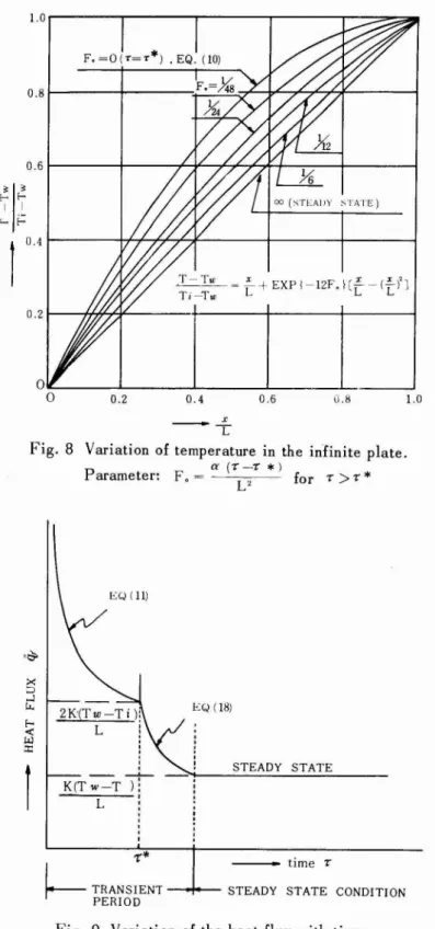
L Tl-lw 0.2 1.0,...---"T""----r---,,....----r---::::::::-:::;;I. 0.81----+---~~~~~ry7".7r---j o.21---fh.~¥_---+_---+_---+----_1 0.61---l---;H~n~'7f+---;-;___+----i x - T

Fig. 8 Variation of temperature in the infinite plate.

P

F'o ~ a (r - r *) * arameter: L' for r

>

r

1

EQ (11) 2K'(Tw-Ti

)!

L

!

, , , , ~

...;;K-'(_T_w~-_T-)

i

L : ,, ,,

,

EQ (18) STEADY STATE

-r*

time r

~

TRANSIENT-oot--- STEADY STATE CONDITION PERIOD

36 Nagata: An Approximate Analysis of Onc~[)imensionalUnsteady State Heat Conduction

Fig. 8 and Fig. 9 show the variati on of the temperature and the heat flux with time in terms of the Fourier Modulus. Mathematically it requires an infinite distance of

time to reach the steady state. Since the term exp {-12F0fhas an effect of damping

the transient temperature distributi00. to the steady state temperature or the linear distribution, and it takes zero at an infinite value of Fourier Modulus. However, we can determine the transient period with sufficient accuracy by adopting a proper value of E ,as example Fo= 1/6, or unity in Fig. 8.

The evaluation of the heat flux in the transient period is obtained by summing up the equation (ll) and (18), the heat flux quantity instantaneously becomes infinitely large, but it converges rafidly to that in the steady state, that is, K(Tw-Ti)/L. The variation of the heat flux is shown in Fig. 9.

The approximate approach discussed so far is helpful to the simplification of the one-dimensional unsteady heat transfer system with constant properties. Especially the evaluation of the temperature and the heat flux in the transient process as pre-steady state are sim plified as discussed in this section.

References

(1) H.Schlichting, "Boundary Layer Theory," McGraw-Hill Book Co., New York, pp138-140 (1960)

(2) T. Nagata, "The Integral Approach to Boundary Layer Flow," Graduate Paper at RPI, Indiana, (1968)

(3) G. Poots, "An Approximate Treatment of a Heat Conduction Problem Involving a Two-Dimensional Solidification Front," Int.

J.

Heat & Mass Trans. Vol. 5, pp 339-348, (1962)

(4)

L.

R. Ingersoll, O.

J.

Zobel, A. C. Ingersoll, "Heat Conduction with Engineering, Geological and Other Applications," The Univ. of Wisconsin Press, Madison, (1954) (5) P.

J.

Schneider, "Conduction Heat Transfer," Addison-Wesley Pub. Co.,