国際系総合研究
C Input-Output Analysis
Lecture 8 IOT (Laos and Nepal)
Katsuhiro SAITO
Department of Agricultural and Resource Economics The University of Tokyo
Structure of Lecture 8
• Review of Input-Output Table and Social Accounting Matrix
• Construction of s SAM (Input-Output Table)
• Application 1 (Resource Based Growth in Lao)
• Application 2 (Impact of Implementation of Current Land Reform Policy in Nepal)
• Talking on the content of next lecture
Review of IO Table and SAM
• Consider an agricultural sector in developing countries. Since it is a
major sector, agricultural policies as well as changes in activities affect all other sectors. Conversely, changes in other sectors might affect
activities in agriculture.
• It is important to capture interaction among sectors and institutions, and an economy-wide analysis or framework is required.
• Input-Output Table and/or Social Accounting Matrix is one of the most powerful source of multi-sectoral analysis.
Review of IO Table and SAM
• Input-Output Analysis
• Basic Model
Open Model: 𝑋 = 𝐴𝑋 + 𝐹 → 𝑋 = (𝐼 − 𝐴)−1𝐹
Closed Model (Income linkage): 𝑉𝑋 = 𝑌 𝑎𝑛𝑑 𝐹 = 𝐹0 + 𝑌𝑓1
• An extension of Basic model: Output Exogenous model 𝑋1 = 𝐴11𝑋1 + 𝐴12𝑋2 + 𝐹1 + 𝐸1 − 𝑀1
𝑋2 = 𝐴21𝑋1 + 𝐴22𝑋2 + 𝐹2 + 𝐸2 − 𝑀2 For example, 𝑋1 is exogenous.
• Price Model
Review of IO Table and SAM
• Input-Output Table is a rectangular array of data which describes the sale and purchase relationships of commodities and services among producers, between producers and consumers within an economy.
• Example (Two sector Input-Output Table)
Source: Miller Blaire Input-Output Analysis, Problems 2.9 in p.66
Review of IO Table and SAM
• Social Accounting Matrix is an extension of Input-Output Table which include income transfers among economic agents (institutions).
• Example (Macro SAM: rearrange of National Income Account)
Macro SAM for LAO, PDR(2001) (Unit: bn kips)
Activities Commodities Factors Firms Households Government Capital ROW Total
Activities 0 27,943 0 0 0 0 0 0 27,943
Commodities 12,241 0 0 0 11,348 1,134 4,927 2,861 32,512
Factors 15,561 0 0 0 0 0 0 0 15,561
Firms 0 0 12,169 0 0 0 0 0 12,169
Households 0 0 3,392 10,755 0 0 0 0 14,148
Government 141 179 0 1,413 368 0 0 1,068 3,169
Capital 0 0 0 0 2,431 2,035 0 462 4,927
ROW 0 4,390 0 0 0 0 0 0 4,390
Total 27,943 32,512 15,561 12,169 14,148 3,169 4,927 4,390 114,819
Source: Author’s estimation.
Review of IO Table and SAM
• Basic Framework of Social Accounting Matrix
• Activities, commodities, factors accounts, current accounts of domestic institutions (households, firms and the gov’t), capital account, the Rest of the World account
1 2 3 4 5 6 7 8 9
Activituy Commodity Factors Firm Household Government Capital ROW Total
1 Activituy Sales Domestic Production
2 Commodity Intermediate Private
Consumption
Gov't
Consumption Investment Export Market Supply
3 Factors Value Added Factor Income
4 Firm Capital
Income Transfer Firm Income
5 Household Labour
Income Divident Transfer Remittance HH Income
6 Government Indirect Tax Tariffs Corporate Tax Income Tax Foreign Grants Gov't Revenue
7 Capital Corporate Savings HH Savings Gov't Savings F.D.I. Total Savings
8 ROW Import Factor Income paid
to ROW
Investment to ROW
Foreign Exchange Outlays
9 Total Production
Cost Absorption V.A. Firm Expenditure HH Expenditure
Gov't Expenditure
Total Investment
Foreign Exchange earning
Review of IO Table and SAM
• Analytical Framework with SAM
• SAM Multiplier Analysis: an extension of IO analysis
• Accounts must be divided into TWO groups (endogenous accounts and exogenous accounts)
•
• CGE(Computable General Equilibrium) Analysis
• Topics in next lecture
Source: Author’s estimation.
Endog. accounts Exog. accounts Total
Endog. accounts 𝑀𝑋 𝐹 𝑋
Exog. accounts 𝐵𝑋 𝐿
Total 𝑋
The matrix of multiplier (𝑰 − 𝑴)−𝟏
The vector of shock ∆𝐹
The vector of impacts ∆𝑋 = (𝐼 − 𝑀)−1∆𝐹
The leakages ∆𝐿 = 𝐵∆𝑋
Construction of a SAM (Input-Output Table)
• Macro SAM constructed from National Income account
• Disaggregating the above Macro SAM: demanding in terms of data
• Activity and commodity balances (Input-Output Table, if available)
• Disaggregation of value added into income by labor categories and profits (employment surveys and sectoral censuses) Sometimes, it is difficult to account for informal sector active
• Determining incomes and outlays of the private institutions and of
households. Household survey, government statistics (transfer between private institutions and gov’t)
• Balancing SAM: RAS method, Cross entropy method
RAS (see https://econo.chukyo-u.ac.jp/yamada/index.html
MTSPIO Excel Macro program written by Prof. YAMADA Mitsuo.
SimSIP-SAM (see https://rotarianeconomist.com/simsip-3/)
Exercise: IO multiplier SAM multiplier
• A SAM for Morocco in 1980 (size: 26X26)
• 11 productive sectors, 5 factors of production (three labor, two capital), 6 households, 1 account for all the firm, gov’t, ROW, capital account.
• Exogenous sectors: gov’t, ROW, capital account: Rest endogenous sectors
• Calculate Input-Output multipliers and Calculate SAM multipliers
• Policy simulations:
• Policy A: Cereal price support (income transfer 100 mil. DH to cereal farmers proportionally to their profit)
• Policy B: increase of Export by 100 mil. DH. Increase export proportionally to the export.
• Policy C: income transfer by 100mil. DH to urban poor household.
• Policy D: income transfer by 100mil. DH to urban rich household.
• Policy E: analyze an income redistribution of 100 mil. DH from the three richest group(urban high, urban middle, and rural hihg) to three poorest group.
Case Study 1: Resource Based Growth in Lao
• Based on Saito,K. Estimating Social Accounting Matrix of Lao PDR and an Evaluation of Resource Based Exportation, Journal of Rural
Economics, Special Issue 2007, 180-187.
• This study is based on SAM of Lao PDR (2001) which is originally estimated by the author.
• Skyline analysis and SAM multiplier analysis are employed.
Overview of Laos
• landlocked by Yunnan in China, Myanmar, Thailand, Cambodia and Viet Nam
• annual per capita GDP in Laos WAS less than 400 US dollars
• population WAS about 5.5 million
• 80% of it is mountainous areas/ total area 236,800km2 /population density is 23 person /km2.
• electricity, garment, wood and its products have comparative advantage
• some of the mineral resources were under development, in recent years
• a few agricultural products were exported
• imports various kinds of goods (domestic supply of consumption and capital goods are poor)
• constant financial deficit and international trade deficit are remarkable
• deficits are difficult to finance by domestic saving, and has been financed by donation and loan from foreign governments
• difficult to invite and improve exporting industries by FDI
• it is realistic to utilize rich natural resource such as water in order to maximize the growth rate
Estimating SAM
• SAM is a square matrix that records transactions between production sectors, agents, and economic institutions at any desired level of
disaggregation
• IO table is a special subset of SAM that describes the production structure of the economy, i.e., transaction of good and services between production sectors.
• Lao Government does not publish SAM, IO table.
Estimating SAM: required data
• Production Cost Structure for each good (Input-Output Table of North East Thailand estimated by Prof. Takanashi)
• Output Value, Value added, Wage,… (UNIDO establishment Survey, Agricultural Statistics )
• Private Consumption, Government Expenditure, Capital Formation, Trade (National Income Statistics)
• Income Source of Household (LECS3 incomplete information)
• Tax Structure(Direct Tax, Indirect Tax, Subsidy, Corporate Tax, Tariff)
• Government Budget (Central Bank of Lao)
Analysis based on estimated SAM
• Input-Output Analysis
• Industrial Structure (Skyline analysis)
• IO multiplier
• SAM Analysis
• SAM multiplier analysis (linear model)
• CGE analysis (non-linear model)
Input-Output Model and Skyline Analysis
( ) ( ) (
1)
X AX F E M X I A
F E M
XF I A1F XE I A1E XM I A1M
Output X is decomposed into XF, XE and XM
X
i X
iF X
iE X
iMXi
XiF 1 XXiE
iF XXiM
iF (total self sufficency ratio)
Exlanation of Skyline analysis
100%
output share of this sector
total sufficeincy ratio
net export
skyline export import
Production share
self sufficiency ratio final demand export import
Skyline of Lao at 2001
1 2 3 4 6 7 8 9 1
0 1 1 1 2 1 3 1 4 1 5 1 6 1 7 1 8
1 9
2 0
2 1
2 2
2 3
2 4
2 5
2 6
0%
20% 40% 60% 80%
100%
200%
300%
400%
500%
600%
700%
800%
900%
1000%
1100%
1200%
See detailed SAM table for the definition of sectors
Findings from the skyline
• agricultural and service sectors are almost self sufficient with little export and import
• other crops (including coffee), textile and its products, wood and wood products, and electricity earn much foreign exchange by its exportation, but the share of these sectors are not so large
• domestic production of heavy and chemical industries cannot fulfill the domestic final demand and much import is required in these sectors.
• Difficult to judge the Laos industrial structure only by one sheet of skyline
• Need to compare w/other year, but we have no other Lao IO table
• As a second best, compare with Thai’s experience
Skyline of Thailand
1 2 3 4 6 811 1
2 1 3
1 1
5 1 6
SSR ImpR
0%
20% 40% 60% 80%
100%
150%
50%
1965
1 2 3 4 56 7 8 9 1
0 1 1
1 2
1 3
1 4
1 5
1 6
SSR ImpR
0%
20% 40% 60% 80%
100%
150%
50%
1970
1 2 3 4 5 6 7 8 9 1
0 1 1 1 2 1 3 1 4 1 5 1 6 1 7 1 8
1 9
2 0
2 1
2 2
2 3 2 4
2 5
2 6
SSR ImpR
0%
20% 40% 60% 80%
100%
150%
50%
1975
1 234 5 6 7 8 9 1 0
1 1 1 2 1 3 1 4 1 5
1 6
1 7
1 8 1 9
2 0
2 1
2 2
2 3 2 4
2 5
2 6
SSR ImpR
0%
20% 40% 60% 80%
100%
150%
200%
250%
50%
2000
Skyline of Thailand 1965
1 2 3 4 6 811 1
2
1 3
1 1
5
1 6
SSR ImpR
0%
20% 40% 60% 80%
100%
150%
50%
Skyline of Thailand 1970
1 2 3 4 56 7 8 9 1
0 1 1
1 2
1 3
1 4
1 5
1 6
SSR ImpR
0%
20% 40% 60% 80%
100%
150%
50%
Skyline of Thailand 1975
1 2 3 45 6 7 8 9 1
0 1 1
1 2 1 3 1 4 1 5
1 6
1 7
1 8
1 9
2 0
2 1
2 2
2 3
2 4
2 5
2 6
SSR ImpR
0%
20% 40% 60% 80%
100%
150%
50%
Skyline of Thailand 2000
1 234 5 6 7 8 9 1 0
1 1
1 2
1 3 1 4 1 5
1 6
1 7
1 8
1 9
2 0
2 1
2 2
2 3
2 4
2 5
2 6
SSR ImpR
0%
20% 40% 60% 80%
100%
150%
200%
250%
50%
Typical Pattern of Industrialization
100%
A B C D Production share
self sufficiency ratio
Skyline analysis of Thailand
First stage 1965-70
• Agriculture, Food manufacturing: large share and exporting sectors
• Manufacturing sector: small share and importing sectors (low sufficiency ratio) Second stage
• Agriculture, Food manufacturing: share is declining, but still exporting sectors
• Manufacturing sector (including capital good): share increasing, self sufficiency ratio is increasing
• Textile: from importing sector to exporting sector
• Typical pattern of Economic development
(Import -> import substitution -> export oriented)
Back to Lao’s skyline
1 2 3 4 6 7 8 9 1
0 1 1 1 2 1 3 1 4 1 5 1 6 1 7 1 8
1 9
2 0
2 1
2 2
2 3
2 4
2 5
2 6
0%
20% 40% 60% 80%
100%
200%
300%
400%
500%
600%
700%
800%
900%
1000%
1100%
1200%
Skyline analysis of Lao
• Large share sectors (agriculture) has almost no export
• Share of exporting sector is about 20%
• Resource based export except for textile
• It is of great idea to improve agriculture as exporting sector if the international commodity market situation permits (for example, maize for feed)
SAM multiplier analysis
• Sectors in SAM are partitioned into two parts: endogenous and exogenous accounts.
• The column coefficients of the endogenous accounts are assumed all to be constant.
• Endogenous accounts are those for which changes in the level of expenditure directly follow any change in income.
• The change in total income or expenditure of each endogenous account w.r.to a unity change in an entry of exogenous account vectors is called SAM multiplier.
SAM multiplier analysis
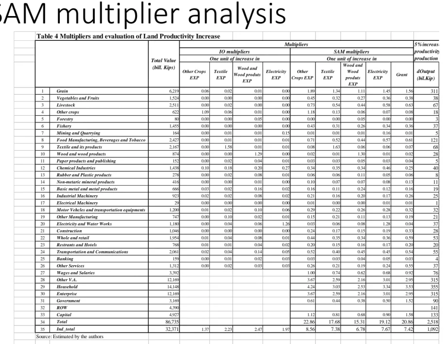
Table 4 Multipliers and evaluation of Land Productivity Increase
Other Crops EXP
Textile EXP
Wood and Wood produts
EXP
Electricity EXP
Other Crops EXP
Textile EXP
Wood and Wood produts
EXP
Electricity
EXP Grant dOutput
(bil.Kip)
1 Grain 6,219 0.06 0.02 0.01 0.00 1.89 1.34 1.11 1.45 1.56 311
2 Vegetables and Fruits 1,524 0.00 0.00 0.00 0.00 0.45 0.32 0.27 0.36 0.38 38
3 Livestock 2,511 0.00 0.02 0.00 0.00 0.73 0.54 0.44 0.58 0.63 67
4 Other crops 622 1.09 0.06 0.01 0.00 1.18 0.13 0.06 0.07 0.08 18
5 Forestry 80 0.00 0.00 0.05 0.00 0.00 0.00 0.05 0.00 0.00 3
6 Fishery 1,455 0.00 0.00 0.00 0.00 0.43 0.31 0.26 0.34 0.36 37
7 Mining and Quarrying 164 0.00 0.01 0.01 0.15 0.01 0.01 0.01 0.16 0.01 5
8 Food Manufacturing, Beverages and Tobacco 2,427 0.00 0.01 0.01 0.01 0.71 0.52 0.44 0.57 0.61 121
9 Textile and its products 2,167 0.00 1.58 0.01 0.01 0.08 1.63 0.06 0.06 0.07 68
10 Wood and wood products 874 0.00 0.00 1.29 0.00 0.02 0.01 1.30 0.01 0.02 28
11 Paper products and publishing 152 0.00 0.02 0.04 0.01 0.03 0.03 0.05 0.03 0.04 5
12 Chemical Industries 1,438 0.10 0.18 0.20 0.27 0.34 0.35 0.34 0.46 0.25 40
13 Rubber and Plastic products 278 0.00 0.02 0.08 0.01 0.06 0.06 0.11 0.05 0.06 8
14 Non-metaric mineral products 416 0.00 0.00 0.01 0.00 0.10 0.07 0.07 0.08 0.13 11
15 Basic metal and metal products 666 0.03 0.02 0.16 0.02 0.16 0.11 0.24 0.12 0.16 19
16 Industrial Machinery 923 0.02 0.02 0.08 0.02 0.21 0.16 0.20 0.17 0.26 25
17 Electrical Machinery 29 0.00 0.00 0.00 0.00 0.01 0.00 0.00 0.01 0.01 1
18 Motor Vehcles and transportation equipments 1,200 0.01 0.02 0.10 0.06 0.29 0.22 0.26 0.28 0.32 32
19 Other Manufacturing 747 0.00 0.10 0.02 0.01 0.15 0.21 0.11 0.13 0.19 21
20 Electricity and Water Works 1,180 0.00 0.04 0.06 1.26 0.03 0.06 0.08 1.28 0.04 37
21 Construction 1,046 0.00 0.00 0.00 0.00 0.24 0.17 0.15 0.19 0.33 28
22 Whole and retail 1,954 0.01 0.04 0.08 0.01 0.44 0.35 0.34 0.36 0.59 53
23 Restrants and Hotels 768 0.01 0.01 0.04 0.02 0.20 0.15 0.16 0.17 0.20 20
24 Transportation and Communications 2,061 0.02 0.04 0.14 0.05 0.52 0.40 0.45 0.45 0.54 55
25 Banking 159 0.00 0.01 0.02 0.03 0.03 0.03 0.04 0.05 0.03 4
26 Other Services 1,312 0.00 0.02 0.03 0.03 0.26 0.21 0.19 0.24 0.55 37
27 Wages and Salaries 3,392 1.00 0.74 0.62 0.68 0.92 76
28 Other V.A. 12,169 3.67 2.59 2.16 3.01 2.95 315
29 Household 14,148 4.24 3.03 2.53 3.34 3.53 355
30 Enterprise 12,169 3.67 2.59 2.16 3.01 2.95 315
31 Government 3,169 0.61 0.44 0.38 0.50 1.52 90
32 ROW 4,390 141
33 Capital 4,927 1.12 0.81 0.68 0.90 1.58 133
34 Total 86,735 22.86 17.68 15.31 19.12 20.86 2,518
35 Ind_total 32,371 1.37 2.23 2.47 1.97 8.56 7.38 6.78 7.67 7.42 1,092
Source: Estimated by the authors
5% increase in Land productivity for rice production Total Value
(bill. Kips)
Multipliers
IO multipliers SAM multipliers
One unit of increase in One unit of increase in
Findings from IO multipliers
• IO multipliers are, in general, smaller than SAM multipliers, and close to zero except for the multipliers of their own sectors.
• Industry sum of multipliers regarding to all industrial sectors (in the last row in the table) are distributed between 1.37 and 2.47.
• Influential sectors are Wood and its products and Textile and its products.
• Electricity is not so much influential to the industrial sectors.
• Other crops that includes coffee has the least input output multiplier among exporting sectors.
• Input output multipliers of agricultural sectors are in general small, due to the inter industry structure of the commodity flow.
Findings from SAM multipliers
• Multipliers for industrial sectors are greater than IO multipliers
• Second, the multipliers regarding to the institutional sectors are greater in value than that of industrial sectors.
• income linkage is stronger if the inter industry transaction is not so developed in the economy like Laos.
• Most influential export sector is the other crops and the next influential sector is the electricity.
• Electricity is important for the Lao economy. Note also that the foreign grant is influential to the economy.
Findings from SAM multiplier: Rice
• We evaluate the impact of 5% increase in land productivity for rice production.
• We assume this happen by the construction of irrigation: reduction of yield instability in wet season and production of rice in dry season. The rice yield is assumed to be increased 5% by technological improvement even without the increase in intermediate inputs of production.
• The activity level of rice milling which is counted as a food manufacturing sector is also stimulated.
• Productivity increase derives 2.7 percent growth in industry output, while it
derives 2.3 to 2.6 increases in wage or other value added such as rent for paddy field.
• Land productivity improvement is of great important for the economy.
• One of the way to improve land productivity is to facilitate irrigation in two
senses; hard and soft. The hard means the physical construction of the irrigation system, while the soft means the development of institutional system such as water use group. In order to have an efficient irrigation system, both of these are crucial.
Implication for development
• While manufacturing sectors are free from natural limitations, agricultural development is restricted by natural conditions and the natural resources.
• To breakthrough the limitation, scientific agriculture such as selective breeding is indispensable.
• Technological progress is necessary for efficient use of scarce resources.
• it is necessary to develop the agricultural sector at first stage of economic development. Why?
(1) the sufficient supply of food is the first priority in the nation
(2) agricultural product (food) is wage commodity and therefore is a cost for manufacturing. The lower, the better.
(3) Agricultural sector supplies labor and capital for the industrialization.
Implication for development: coffee
• Though SAM multiplier is surely large, another consideration is necessary whether this is preferable for economy.
• export of agricultural commodity is important for foreign exchange earning, but the international price fluctuation of primary
commodities is also large
• export price declining may have negative influence on the economic growth (Prebisch and Singer Hypothesis).
• high SAM multiplier means that impact of a change in international price is magnified to the domestic economy.
• It is recommended to avoid export specialization of a few of specific commodities and to reduce the price risk for exportation by
increasing the variety of export commodities.
Implication for development: electricity
• Since LAOS is water resource abundant country, it has a comparative advantage for producing and export electricity (supply side condition).
• The neighbor countries who enjoy high economic growth rate show high demand for energy (demand side condition).
• hydraulic power generation is preferable in terms of the environment (GHG)
• If export is determined by a long period contract basis, export price is rather stable.
• It is often said that dam construction for hydraulic power generation surely lead to the environmental disruption of Laos. From a viewpoint of economics, it is the fact that we must pay a cost to obtain some
benefit (Do not underestimate environmental damage).
Appendix
Spillover of sectoral productivity increase
Welfare Impact of 5% increase in TFP in each sector (%)
Thailand Vietnam Cambodia Laos ROW GDP Share (2000)
21,835 5,050 848 289 5,687,691
Agriculture 0.40 0.00 0.00 0.00 0.0 9.0
Manufacture 1.40 0.10 0.10 0.10 0.0 42.0
Service 2.39 0.20 0.20 0.10 0.0 49.0
Agriculture 0.10 1.10 0.00 0.00 0.0 24.5
Manufacture 0.10 0.80 0.00 0.00 0.0 36.7
Service 0.10 1.69 0.00 0.00 0.0 38.7
Agriculture 0.00 0.00 1.19 0.00 0.0 39.6
Manufacture 0.00 0.00 0.90 0.00 0.0 23.3
Service 0.10 0.00 1.79 0.00 0.0 37.1
Agriculture 0.00 0.00 0.00 2.69 0.0 55.2
Manufacture 0.00 0.00 0.00 0.80 0.0 27.3
Service 0.00 0.00 0.00 0.60 0.0 24.6
Agriculture 0.00 0.00 0.10 0.00 0.3 5.5
Manufacture 0.20 0.20 0.20 0.00 1.1 21.5
Service 0.30 0.20 0.30 0.00 3.5 73.0
Source: Authors' estimation by using LMB ICGE model.
Thailand
Vietnam
Benchmark Utility Index
Cambodia
Laos
ROW
Case Study 2: Land Policy evaluation in Nepal
• Based on Damaru Ballabha Paudel and K. Saito Impact of Implementation of Current Land Reform Policy in Nepal, Japanese Journal of Rural Economics 17, 2015, 35-39.
• This study is based on SAM of Nepal(2010/11) which is originally estimated by the authors.
• Simulation Analysis based on SAM is conducted.
• Scenario is based on our previous study:
• Paudel,D.B. and K. Saito An Evaluation of Land Reform in Nepal -Simulation Based Approach, Japanese Journal of Rural Economics, Special Issue 2012,418-425.
• Paudel, D. B. and K. Saito, Does Land Reform Increase Efficiency in a Developing Economy? A Case from Nepal, Department of Agricultural and Resource
Economics Working Paper Series 13-E-001, The University of Tokyo, 2013.
Introduction
• Low economic growth and high prevalence of poverty are the inherent features of Nepalese economy.
• The economic growth was about 4% for last decade (Ministry of Finance [7]) and the absolute poverty in 2011 was 25.2% (Central Bureau of Statistic [4]).
• As average productivity of cereals crops is 2.85 metric tons per hectors (The World Bank [13]), it is the lowest in South Asian Region.
• Additionally, only 17% of the country’s total land is arable and ownership distribution of land is skewed.
Introduction
• The visible inequality in land distribution is one of the causes of low productivity in Nepal because those who have farming skills do not have enough land and those who have land do not have farming skill or no necessity of farming (Adhikari and Bjondal [1]).
• This kind of adverse situation in land is causing a vocal demand for land reform.
• However, Nepalese land reform was started in 1951 and
comprehensive land reform law was commenced in 1964, the progress of land reform is very slow.
Introduction
• Many studies (Regmi [12]; Community Self-Reliance Centre, [5];
Adhikari [2]; Adhikari and Bjorndal [1] etc.) evaluated the land reform process of Nepal as unsuccessful so far and indicated the need for
successful land reform.
• Moreover, land reform issues are live issues in many developing
countries including Nepal (Lipton [ 6]) and they are more serious now than decades ago because land reform has not come to a logical end and the story of poverty and inequality is much more complex today.
• Therefore, we, in this paper, evaluate the potential impact of land reform in Nepal using social accounting matrix (SAM) framework.
Introduction
• If the current land ceiling provisions were implemented strictly, what would be the impact of land reform on income distribution of households; and in the whole economy; is the main research purpose in this study.
• Thus, to fulfill this research purpose, we make different three scenarios for land reform and see the effect of reform in
production, households income and the whole economy.
• Here, we intend to see the micro-simulation effect of land reform on macro-economy of Nepal, which is also the distinct feature of this study.
• To the best of our knowledge, this type of micro-simulation macro-effect study is new in literature.
Nepal SAM 2010/11 and Its Features
• In this paper, we use Nepal SAM 2010/11 (Paudel and Saito [11]) as main source of data.
• In this SAM, activities and commodities are divided into 36 sectors
which include 12 sectors for agriculture, 11 sectors for manufacturing and rest 13 sectors for construction, trading, services and others.
• Similarly, three primary factor accounts (land, labor, capital) and four government accounts - income tax, value added tax, import tariff,
other government activities; one enterprise account, one capital account, and one rest of the world account.
Nepal SAM 2010/11 and Its Features
• Average share of labor income is higher in urban households (37.83%) than rural (23.37%).
• Similarly, urban households have average share of capital rental income (9.07%) higher than rural households do (5.20%). However, share of other sources of income (land rental income, business enterprise income,
government transfer income and foreign exchange income or remittance income) is higher in rural households.
Nepal SAM 2010/11 and Its Features
• Average share of consumption expenditure on commodities is higher in rural households (90.54%) than urban (74.79%).
• However, share of taxes to government is higher in urban households (4.42%) than rural (0.45%). Similarly, share of saving is higher in urban households (20.79%) than rural (9.02%).
Impact of Land Reform
• In case of Nepal, the Land Related Act 1964 (Nepal Law Commission [8]) is the main law for land reform. It is amended many times and the
mentionable amendment is the Fifth Amendment.
• The Fifth Amendment to the Land Related Act 1964 was done in 2002 (hereafter, FALRA 2002) that drastically reduced the land ceiling in the country aiming to use land in the most productive way.
• According to FALRA 2002, land ceiling was reduced as follows including both agricultural and homestead land.
Region Ceiling reduction Reduction rate
Terai 18.40 ha to 7.45 ha 60%
Kathmandu Valley 3.10 ha to 1.52 ha 51%
Other regions 4.90 ha to 3.81 ha 22%
Impact of Land Reform
• The law made provision of redistributive land reform in favor of poor farmers but the law could not come into action due to many barriers from opposing forces including deficiency of proper implementation of policy.
• Land reform in Nepal has always been criticized for lack of will power to implement it (Regmi [12]).
• FALRA 2002 also was not properly implemented indicating failed
reform on land. The scenario of land distribution would be different if the land ceiling policy of FALRA 2002 were properly implemented
(Paudel and Saito [9]).
Impact of Land Reform
• Moreover, having more household land shows a higher status in society,
more influence in politics and it also helps as collateral for borrowing credit.
• Paudel and Saito [9] estimated consumption function and found that transfer of beyond ceiling land from large holdings to marginal and
landless will not only change the structure of land ownership but also the consumption pattern in Nepalese economy.
• The mean per capita consumption of large households will decrease but per capita consumption of landless and marginal households increase substantially.
• Consequently, using household level survey data (Central Bureau of
Statistics [3]), they estimated that how implementation of redistributive land reform affects per capita consumption of households (see table 3).
Impact of Land Reform
Impact of Land Reform
• Likewise, Paudel and Saito [10] also estimated stochastic frontier function for Nepalese agriculture and found that household farms are operating less than frontier and inefficiency sources are common.
• Besides, the gap between frontier and actual production is 30% and mean technical efficiency scores vary widely between household land sizes and regions. According to them, if land reform policies were implemented and inefficiencies were eliminated, the agricultural productivity would rise
even using the same level of inputs.
• Furthermore, utilization of unused land and consolidation of fragmented land could reduce at least 10% of inefficiency in Nepalese agriculture.
Therefore, for simulation purpose, we assume 10% productivity can be raised by eliminating some of the inefficiencies. We term this type of reform as productivity augmenting reform in this study.
Framework for analysis
(1) 𝑿 = 𝑨𝑿 + 𝑭 (3) 𝚫𝑿 = 𝑴𝚫𝑭
(2) 𝑋 = (𝐼 − 𝐴)−1𝐹 = 𝑀𝐹 (4) ∆𝐿 = 𝐵∆𝑋
• Model
• X: vector of total income or expenditure of the endogenous accounts (ΔX : the vector of impacts)
• F: vector sum of the expenditures of the exogenous accounts (ΔF: the vector of shocks)
• L: column vector of the income of exogenous accounts (ΔL: the leakages)
• A: a square matrix of coefficients of endogenous accounts, B: a rectangular matrix of coefficients with exogenous accounts, M:
multipliers.
• Endogenous Accounts: Activities, Commodities, Factors, Enterprises, Households
• Exogenous Accounts: Government Accounts, Capital Accounts, Rest of the World Accounts
• Moreover, in this model we treat land endowment as policy variable (as exogenous variable) while land input is one of the factors of production and endogenous variable. Land input is the total operated land in the economy while land endowment is total owned land. Land endowment also includes unused land such as left fallow land.
Framework for analysis: Scenarios
• Simulation 1: distributive land reform
• Because of the implementation of current ceiling policy, i.e., FALRA 2002, the large households lose their beyond ceiling land but landless and marginal households will receive land.
• We simulate this change within the household categories in this scenario and see the direct and induced impacts of land reform. For this simulation, we assume that the households, which either gain or lose their income as the result of land reform, are exogenous.
• Simulation 2: 10% increase in crops sector production
• We assume that if productivity-augmenting land reform were implemented, at least 10%
productivity of agricultural sectors (crops productivity) would rise.
• Eliminating mainly two barriers- utilizing the unused land and reducing land fragmentation would gain this productivity. In this simulation, we assume that crop production activities are exogenous;
other activities are
• Simulation 3: simulation 1 and simulation 2 simultaneously
Results and Discussions
Results and Discussions
• From Table 4,
• Redistributive reform (simulation 1) is pro-poor reform because it has more impact on rural income than on urban income.
• Production augmenting reform (simulation 2) has higher impacts on economy. Both reforms together (simulation 3) has the highest
impacts on production, income, revenue, savings, foreign exchange and employment.
Results and Discussions
Results and Discussions
• Comparing between three policy scenarios given by three simulations, we clearly see that 10% productivity augmenting reform (Simulation 2) has higher impacts that redistributive reform (Simulation 1) and both reforms simultaneously (simulation 3) have the highest impacts among the three alternative policies.
• For rural income, simulation 1 has higher impacts than simulation 2.
Results and Discussions
Results and Discussions
Results and Discussions
• Paddy, wheat and other grains & crops sectors are kept exogenous in simulation 2 and 3 and they have constant impacts of 10% while
other have variable impacts.
• Impacts of simulation 3 are higher than simulation 1 and 2. Impacts of simulation 2 are higher in most of the cases except forestry and food processing sectors
Results and Discussions
• This figure show the impacts of land reform on factor income. All the
simulations have highest impact on land income.
Results and Discussions
Results and Discussions
Results and Discussions
• Landless and marginal households gain from redistributive reform, while large households lose.
• Gain is higher than lose and overall household income increases.