Cauchy Aperture and Perfect Reconstruction Filters for Extending Depth-of-Field from Focal Stack

(1)

PAPER

Special Section on Picture Coding and Image Media Processing

Cauchy Aperture and Perfect Reconstruction Filters for Extending Depth-of-Field from Focal Stack

Akira KUBOTA^†a), Kazuya KODAMA^††,Members,andAsami ITO^†,Nonmember

SUMMARY A pupil function of aperture in image capturing systems is theoretically derived such that one can perfectly reconstruct all-in-focus image through linear filtering of the focal stack. The perfect reconstruction filters are also designed based on the derived pupil function. The designed filters are space-invariant; hence the presented method does not require region segmentation. Simulation results using synthetic scenes shows eﬀec- tiveness of the derived pupil function and the filters.

key words: extended depth-of-field, focal stack, aperture, perfect recon- struction filters, image fusion

1. Introduction

Depth-of-Field (DOF) of an imaging system is the depth range in which scenes appear in-focus in the captured image. Most imaging systems, especially in microscopy, have narrow DOF; hence the captured images suﬀer from blur- ring in the regions which depths are not in the DOF. In order to obtain the all-in-focus images where all the regions are in-focus, extensive methods for extending DOF have been studied in the last decades. These methods are categorized into two groups: image recovery from a single captured image and image fusion using multiple captured images.

In image recovery approaches, so called blind image recovery[1], an all-in-focus image is to be recovered from a single captured image. The captured image, sayg(x, y), is modeled as

g(x, y)=

h(x, y,p,q)f(p,q)d pdq, (1) where f denotes the desired all-in-focus image, h point- spread-function (PSF) and (x, y) image coordinates. Since PSF h is unknown and space-variant (varies with scene depth), it is generally diﬃcult to estimate f with adequate quality for arbitrary scenes without some priors on imagef. Recently, to robustly recover f, some techniques[2]–

[5]have been presented based on designs of optics in imaging system. These methods can make PSFs space-invariant by putting special optical elements at the aperture plane.

The model of the imaging process is expressed by convolution of f andh:

Manuscript received February 17, 2019.

Manuscript revised June 9, 2019.

Manuscript publicized August 16, 2019.

†The authors are with Chuo University, Tokyo, 112–8551 Japan.

††The author is with National Institute of Informatics, Tokyo, 101–8430 Japan.

a) E-mail: [email protected] DOI: 10.1587/transinf.2019PCP0006

g(x, y)=

h(x−p, y−q)f(p,q)d pdq; (2) hence the all-in-focus image f can be recovered simply by deconvolvinggwithout involving depth estimation.

This space-invariant imaging can be also achieved by focus sweep methods[6]–[8], where an image was captured over moving the sensor plane during the exposure time. The PSF of the captured image, called integrated PSF, is shown to be nearly space-invariant and therefore the imaging model is expressed by Eq. (2).

The other category is image fusion[9]–[16]. Unlike above deconvolution methods using a single captured image, image fusion methods capture multiple images with different focus depths (a set of them is called focal stack) and fuse them into the all-in-focus image. Because scene textures at any depth appear in-focus in one of the focal stack images, much robust recovery is possible. Image fusion methods consist of two parts. The first part is to se- lect dominant values from pixel values in the spatial domain or dominant coefficients in the transformed domain. The second part is to combine these selected values/coefficients into the fused image. These methods are essentially same as region segmentation; hence often suffer from blocking ar- tifacts due to incorrect regions estimations. In addition, a key to high-quality fusion is the selection rule[17], based on which true values/coefficients of the all-in-focus image can be correctly selected; however, it is difficult to design the selection rule for perfect reconstruction.

To tackle these problems above, this paper presents a novel filter-based image fusion method for reconstructing an all-in-focus image f from focal stack, say{g₁, g₂, . . . , gN}, by

f(x, y)=

N

i=1

ki(x, y)∗gi(x, y), (3) where the operation∗denotes two-dimensional convolution and the set of filterski(i=1,2, . . . ,N) is the synthetic filter bank. In this paper, the pupil function of the aperture in image capturing systems is derived such that one can perfectly reconstruct all-in-focus image by Eq. (3) in theory. The filter bank is also designed based on the derived pupil function.

The designed filters are all space-invariant; hence the presented method requires neither depth estimation nor region segmentation.

For the case of N = 2, the author derived synthetic filters that perfectly reconstruct all-in-focus image[18]. It Copyright c2019 The Institute of Electronics, Information and Communication Engineers

(2)

is possible to show the existence of the filters for normally used pupil functions such as Gaussian and pill-box functions. Extending this idea to the case ofN ≥ 3, however, does not lead stable filters; hence an iterative reconstruction method[19],[20]and regularization method[21]have been applied for this case. But, they estimate focus slice images (in-focus regions) and do not derive filters that perfectly reconstruct the all-in-focus image directly from the focal stack. In this paper, to achieve perfect reconstruction, the pupil function is theoretically designed. In practice, the focal stack should be captured by a specially designed camera with the aperture of the presented pupil function.

Some filtering approaches to all-in-focus image reconstruction have been presented. The authors[22],[23]presented three-dimensional deconvolution method in the Fre- quency domain that recovers the all-in-focus image from the focal stack. They[25]and Levin et al.[26]showed that this approach is achieved by two-dimensional filtering of the averaged image of the focal stack, which is the same with focus sweep method. However, the imaging models of the focal stack or its average used in these methods are approx- imations of the accurate version; for robust reconstruction, the focusing range must be set wider than the actual depth range of the scene.

Designing pupil functions of the aperture, called coded aperture, has been recently studied in depth-from-defocus methods[27]–[29]that use a few images captured with different focus depths to reconstruct shape of scenes as well as all-in-focus image. But, in image fusion methods, eﬀect of pupil function and its optimal design have not been well studied.

This paper is an extended version of the paper in[30].

In this paper, the performance evaluations of reconstruction accuracy and noise sensitivity are additionally discussed in detail.

2. Cauchy Aperture and Perfect Reconstruction Filters

2.1 Imaging Model 2.1.1 Focal Stack Model

A focal stack is a set of images captured by changing the distance of the imaging plane from the lens with equal interval. Letg_i(x, y) be the image captured when the distance isvi (i = 1,2, . . . ,N). The coordinate (x, y) represents the image coordinate perpendicular to the optical axis. Here we assume thatv₁ > v₂ >· · ·> vN holds and the magnification diﬀerence is already corrected among the captured images.

H=

⎛⎜⎜⎜⎜⎜

⎜⎜⎜⎜⎜

⎜⎜⎜⎝

1 A(tξ,tη;σ) A(2tξ,2tη;σ) . . . A((N−1)tξ,(N−1)tη;σ) A(tξ,tη;σ) 1 A(tξ,tη;σ) . . . A((N−2)tξ,(N−2)tη;σ)

A(2tξ,2tη;σ) A(tξ,tη;σ) 1 ... ...

... ... ... ... A(tξ,tη;σ)

A((N−1)tξ,(N−1)tη;σ) A((N−2)tξ,(N−2)tη;σ) . . . A(tξ,tη;σ) 1

⎞⎟⎟⎟⎟⎟

⎟⎟⎟⎟⎟

⎟⎟⎟⎠

. The pupil function is assumed to be circularly symmetric and expressed bya(x, y;σ) with a scaling parameterσthat determines the amount of blur degree. It should satisfy the condition of

⎧⎪⎪⎨

⎪⎪⎩

a(x, y;σ)dxdy=1

a(x, y;σ)≥0 . (4)

Let fi(x, y) be the in-focus regions in the captured imagegi(x, y) and call it focus slice image. The focal stack is modeled by combination of the focus slices[18]–[21],[31]

as

gi(x, y)=

N

j=1

hi j(x, y)∗ fj(x, y), i=1,2, . . . ,N, (5) where∗denotes two-dimensional convolution and the func- tionhi j(x, y) represents a point spread function (PSF), which is a scaled version of the pupil function

hi j(x, y)

=

⎧⎪⎪⎪⎪⎪⎨

⎪⎪⎪⎪⎪

⎩ 1

|i−j|²t²a

x

|i−j|t, y

|i−j|t;σ

(i j)

δ(x, y) (i= j)

. (6)

The parameter t is a ratio of the distance interval of the image plane to the focus length and δ(x, y) is the two- dimensional Dirac delta function.

The model in Eq. (5) is represented in the Fourier domain in matrix-vector form:

g=Hf, (7)

where

g=

⎛⎜⎜⎜⎜⎜

⎜⎜⎜⎜⎜

⎝

G1(ξ, η) G2(ξ, η)

... GN(ξ, η)

⎞⎟⎟⎟⎟⎟

⎟⎟⎟⎟⎟

⎠

, f =

⎛⎜⎜⎜⎜⎜

⎜⎜⎜⎜⎜

⎝

F1(ξ, η) F2(ξ, η)

... FN(ξ, η)

⎞⎟⎟⎟⎟⎟

⎟⎟⎟⎟⎟

⎠ ,

andH(see equation at the bottom).

In the above equation, functionsGi,Fi andAdenote the Fourier transform ofgi, fianda, respectively, and (ξ, η) is spatial frequencies. Note that the matrixHis a symmetric Toeplitz matrix.

2.1.2 All-in-Focus Image Model

The all-in-focus image f(x, y) is represented by a sum of the focus slice images fi(x, y):

(3)

f(x, y)=

N

i=1

fi(x, y). (8)

Its Fourier transform is written in vector form by

F(ξ, η)=1^T_Nf, (9)

whereFis the Fourier transform of f,1Nis defined by aN- dimensional vector which elements are all 1, andT denotes the transpose operation.

2.2 Deriving Synthetic Filters and Pupil Function

Eliminating the focus slice images f from Eqs. (7) and (9) yields

F(ξ, η)=(1^T_NH⁻¹)g. (10)

If the column vector1^T_NH⁻¹ exists, each element gives the frequency characteristicKiof the filterkito the imagegi.

A suﬃcient condition such that1^T_NH⁻¹exists is that the matrixHshould become the form of Kac-Murdock-Szeg¨o matrix[32](see the matrix H_KMS at the bottom). In short, sinceHis symmetric, this condition is written by

A(|i−j|tξ,|i−j|tη;σ)=A^|ⁱ⁻^j^|(tξ,tη;σ). (11) IfHsatisfies this condition,H⁻¹exists for the case of A(tξ,tη;σ)1 (as shown in the matrixH⁻¹at the bottom) and Eq. (10) can be represented by

F(ξ, η)= 1

1+A(tξ,tη;σ)(G1+GN) +1−A(tξ,tη;σ)

1+A(tξ,tη;σ)(G₂+· · ·+GN−1). (12) It is found that the frequency characteristics of the filters are obtained to be

Ki(ξ, η)=

⎧⎪⎪⎪⎪⎪⎪⎨

⎪⎪⎪⎪⎪

⎪⎩

1

1+A(tξ,tη;σ) (i=1,N) 1−A(tξ,tη;σ)

1+A(tξ,tη;σ) (i=2,3, . . . ,N−1) (13)

HKMS=

⎛⎜⎜⎜⎜⎜

⎜⎜⎜⎜⎜

⎜⎜⎜⎝

1 A(tξ,tη;σ) A²(tξ,tη;σ) . . . A^N⁻¹(tξ,tη;σ) A(tξ,tη;σ) 1 A(tξ,tη;σ) . . . A^N⁻²(tξ,tη;σ) A²(tξ,tη;σ) A(tξ,tη;σ) 1 ... ...

... ... ... ... A(tξ,tη;σ)

A^N⁻¹(tξ,tη;σ) . . . A(tξ,tη;σ) 1

⎞⎟⎟⎟⎟⎟

⎟⎟⎟⎟⎟

⎟⎟⎟⎠

H⁻¹= 1 1−A²(tξ,tη;σ)

⎛⎜⎜⎜⎜⎜

⎜⎜⎜⎜⎜

⎝

1 −A(tξ,tη;σ)

−A(tξ,tη;σ) 1+A²(tξ,tη;σ) −A(tξ,tη;σ)

... ... ...

−A(tξ,tη;σ) 1+A²(tξ,tη;σ) −A(tξ,tη;σ)

−A(tξ,tη;σ) 1

⎞⎟⎟⎟⎟⎟

⎟⎟⎟⎟⎟

⎠

Fig. 1 Characteristics of Cauchy aperture function (the maximum ampli- tude is normalized to 1).

and that they are stable even for the case ofA(tξ,tη;σ)=1.

Therefore, all the filters exist for all the frequencies and are stable reconstruction filters.

The functionAthat satisfies the condition (11) in addition to the condition (4) is an exponential function of

A(ξ, η;σ)=exp

−2πσ ξ²+η²

; (14)

hence its inverse Fourier transform gives the pupil function in spatial domain as

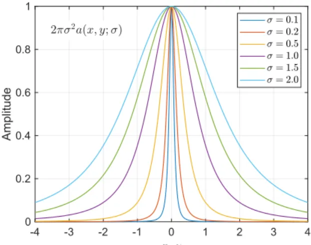
a(x, y;σ)= σ

2π(x²+y²+σ²)^3/2. (15) This is two-dimensional Cauchy distribution function[33].

We call this pupil function Cauchy aperture function in this paper. The examples of the function are plotted in Fig. 1.

Figure 2 shows the frequency characteristics of the filters forσ = 1.0. This indicates that all the filters work as high-pass filters and extract higher frequency components corresponding to the in-focus regions from the focal stack to reconstruct the all-in-focus image. The direct current and lower frequency components of the all-in-focus image were compensated from the first and the last focal stack images.

(4)

Fig. 2 Frequency characteristics of synthetic filters and Cauchy PSF of σ=1.0.

2.3 Advantages and Disadvantages

The advantage of the presented method is that the presented method can reconstruct all-in-focus image perfectly without requiring region segmentation, which means it is indepen- dent of the target scenes.

The presented method has mainly two disadvantages.

The first is that noise in the focal stack images are accumu- lated in the reconstructed images. This eﬀect will be theoretically and numerically evaluated in Sect. 3. The other is that the imaging model of focal stack images is in practice not correct for the occluding boundaries; therefore the presented method causes errors for those regions when using real captured focal stack images.

3. Simulation

3.1 Preparation of Ground Truth and Focal Stack Images Three test images of “Baboon”, “Lenna” and “Peppers”

were used as the ground truth of all-in-focus imagef. These test images are 24-bit color images with 512×512 pixels.

The focal stack imagesg_i (i = 1,2, . . . ,N) were synthet- ically generated based on the imaging model (7) using the focus slice imagesfiwhich were created by equally dividing the ground truth intoNthin rectangles from the left edge.

In this simulation, the maximum of the blur amount in the focal stack images, (N−1)σt, was fixed to 10 [pixels], which means the depth range of the synthetic scene is fixed.

Under this condition, the number of depth layers, N, were changed to 8, 16, 32 and 64. (See some examples of the focal stack images generated in Figs. 4 and 5)

3.2 Evaluation of Perfect Reconstruction

To precisely evaluate whether the presented method achieves perfect reconstruction, we calculated root mean squared error (RMSE) of the reconstructed images in double

Table 1 RMSEs of reconstructed all-in-focus images in double precision for “Peppers” test image.

Method Number of depth layers,N

8 16 32 64

Presented (×10⁻¹³) 1.09 1.13 1.10 1.09 focus sweep[25],[26](×1) 23.7 6.35 5.57 5.56

Fig. 3 RMSEs of focus slices for “Peppers” test image.

precision floating-point number. In this evaluation, we used the focal stack images that were stored in double precision without 8-bit quantization.

The results for “Peppers” image are shown in Table 1.

All the RMSEs are quite small and less than 10⁻¹², indicat- ing that perfect reconstruction can be achieved by the presented method. For comparison, RMSEs of the focus sweep method were also calculated in double precision. As shown in Table 1, the RMSEs are much larger in comparison to those of the presented method. This shows that the focus sweep method cannot perfectly reconstruct all-in-focus images.

Figure 3 (a) and (b) show RMSEs of the focal slice regions in the presented and the focal sweep methods respectively for the case of N = 64. These results found that the presented method has almost constant RMSEs around 1.1×10⁻¹³over all depths. In contrast, RMSEs of the focus sweep method vary according to depths and is increased at depths far from the middle. This is due to the modeling error of the averaged focal stack image.

3.3 Evaluation of Noise Sensitivity

Since the presented filtering process is linear, its noise sensitivity can be quantitatively evaluated when the additive

(5)

noise is white. We here define noise amplification factor (NAF) as the metric of noise sensitivity byRMSE/σn, where RMSErepresents RMSE of the reconstructed image andσn

the standard deviation of the additive noise. In this simulation, the NAF of the presented method is given by

NAF=

1

512² 511 k=0

511 l=0

N

i=1

|Ki(k,l)|², (16) whereKi(k,l) denote the discrete Fourier transform of the synthetic filters and (k,l) the indices of spatial frequencies.

Similarly, for the focus sweep method, the NAF can be given by

NAF=

1

512²·N 511

k=0

511 l=0

|D(k,l)|², (17) whereD(k,l) denotes the discrete Fourier transform of the deconvolution filter. Note that the noise standard deviation is reduced toσn/√

Nbecause the average image of the focal stack images is computed.

The NAFs computed for both presented and focus sweep methods are shown in Table 2. In the simulation settings, all the NAFs of the presented method are less than 3, which indicates the presented method is not so sensitive to noise as most image recovery methods have in usual. This is because the presented filters are stable and the frequency characteristics have 1 at a maximum as shown in Fig. 2. On the other hand, forN = 8,16,32, the focus sweep method has higher NAFs and more sensitive to noise than the presented method. But, for N = 64, thanks to the averaging eﬀect, the NAF is decreased and is lower than that of the presented method.

Table 3 shows the NAFs calculated using the reconstructed images from the focal stack images with white Gaussian noise ofσn = 10 and 20. When calculating the NAF, we used the reconstructed images and the focal stack images after unsigned 8-bit quantization. The calculated

Table 2 Noise amplification factorsRMSE/σn.

method Number of layers,N

8 16 32 64

Presented 2.56 2.72 2.32 1.78

focus sweep[25],[26] 10.9 4.05 2.44 1.64

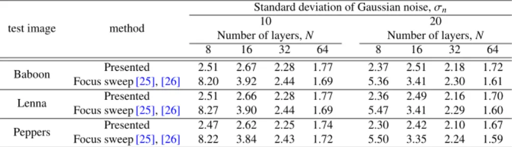
Table 3 Calculated noise amplification factors using three test images in presence of white Gaussian noise.

test image method

Standard deviation of Gaussian noise,σn

10 20

Number of layers,N Number of layers,N

8 16 32 64 8 16 32 64

Baboon Presented 2.51 2.67 2.28 1.77 2.37 2.51 2.18 1.72

Focus sweep[25],[26] 8.20 3.92 2.44 1.69 5.36 3.41 2.30 1.61

Lenna Presented 2.51 2.66 2.28 1.77 2.36 2.49 2.16 1.70

Focus sweep[25],[26] 8.27 3.90 2.44 1.69 5.47 3.41 2.29 1.60

Peppers Presented 2.47 2.62 2.25 1.74 2.30 2.42 2.10 1.67

Focus sweep[25],[26] 8.22 3.84 2.43 1.72 5.50 3.35 2.24 1.59

NAFs are similar to the theoretical values in Table 2. For the case ofN=8 in the focus sweep method, the NAFs are lower than the theoretical values because of the clipping at 0 and 255 in the quantization.

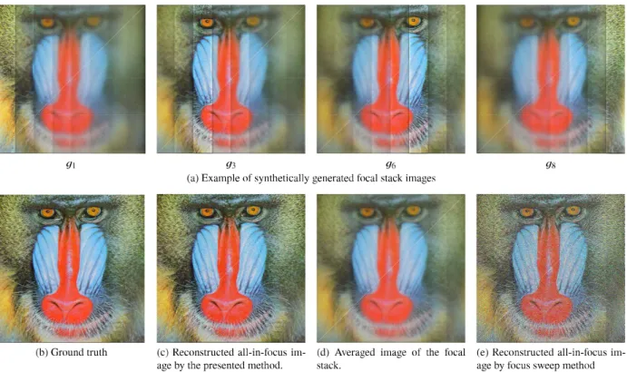
Figure 4 shows the simulation results using “Baboon”

test image forN =8 andσn =10. As shown in Fig. 4 (a), the focal stack images were generated from the ground truth image (Fig. 4 (b)). Each focal stack image consists of eight regions in diﬀerent focus settings. For example, the image g₁is focused on the nearest region (the most left rectangle) and is out of focus in the other regions; the imageg₈is focused on the farthest region (the most right rectangle) and is out of focus in the other regions.

The all-in-focus image reconstructed by the presented filter bank is shown in Fig. 4 (c). It can be seen that the reconstructed image appears in-focused on all eight regions and is close to the ground truth except the region boundaries.

The noise in the reconstructed image is amplified by 2.51 times (see Table 3), but this is not severe quality degrada- tion. For comparison, the all-in-focus image reconstructed by the conventional focus sweep method[25],[26]is shown in Fig. 4 (e), which is deconvoluted from the averaged image (Fig. 4 (d)) of the focal stack. In this result, noise is amplified by 8.20 times and the quality is degraded.

The another simulation results using “Peppers” test image forN=64 andσn=20 are shown in Fig. 5. Figure 5 (a) shows examples of the focal stack images generated from the ground truth image in Fig. 5 (b). The generated focal stack images have continuously 64 depth regions with different focus eﬀects. As shown in Fig. 5 (c), the reconstructed image by the presented filter bank looks in-focus over all the regions. The noise is amplified only by 1.67 and the quality is not much degraded compared with that in the focal stack images. Figure 5 (e) shows the all-in-focus image reconstructed by the focus sweep method[25],[26]from the averaged focal stack image (Fig. 5 (d)) Although the focal slices in middle layers are recovered in-focus, the nearest and the farthest regions are slightly blurry compared to the ground truth. This is because PSF of the averaged image is approximately modeled to be space-invariant PSF.

As future work, to suppress noise amplification, noise reduction of the focal stack is needed. Some robust noise reduction methods for video data will be eﬀective, since a set of the focal stack images is a 3D data same as video data.

(6)

Fig. 4 Simulation results using “Baboon” test image forN=8 andσn=10.

Fig. 5 Simulation results using “Peppers” test image forN=64 andσn=20.

4. Conclusion

The aperture function was theoretically derived as 2D Cauchy function for perfectly reconstructing all-in-focus

image by filtering the focal stack images. The filters were simply designed using the function. In the simulation, the all-in-focus image was successfully reconstructed with high quality by the presented filters without region segmentation.

In future, we will evaluate the performance of the pre-

(7)

sented method through experiments using real captured focal stack images. To do this, we need to design not only aperture but also lens system to create Cauchy PSF as precisely as possible on the captured focal stack. In addition, extending to producing re-focusing and perspective shifting eﬀects will be considered.

References

[1] D. Kundur and D. Hatzinakos, “Blind image deconvolution,” IEEE Signal Process. Mag., vol.13, no.3, pp.43–64, 1996.

[2] E.R. Dowski and W. Cathey, “Extended Depth of Field Through Wavefront Coding,” Applied Optics, vol.34, no.11, pp.1859–1866, 1995.

[3] S. Bradburn, W.T. Cathey and E.R. Dowski, “Realizations of focus invariance in optical–digital systems with wavefront coding,” Appl.

Opt., vol.36, no.35, pp.9157–9166, 1997.

[4] N. George and W. Chi, “Extended Depth of Field Using a Log- arithmic Asphere,” J. Optics A: Pure and Applied Optics, vol.5, pp.157–163, 2003.

[5] A. Castro and J. Ojeda-Castaneda, “Asymmetric Phase Masks for Extended Depth of Field,” Applied Optics, vol.43, no.17, pp.3474—3479, 2004.

[6] G. H¨ausler, “A Method to Increase the Depth of Focus by Two Step Image Processing,” Optics Comm., vol.6, no.1, pp.38–42, 1972.

[7] S. Kuthirummal, H. Nagahara, C. Zhou, and S.K. Nayar, “Flexible Depth of Field Photography,” IEEE Transactions on Pattern Recog- nition and Machine Intelligence, vol.33, no.1, pp.58–71, 2011.

[8] D. Miau, O. Cossairt, and S.K. Nayar, “Focal sweep videography with deformable optics,” IEEE International Conference on Compu- tational Photography, pp.1–8, 2013.

[9] H.A. Eltoukhy and S. Kavusi, “A computationally eﬃcient algo- rithm for multifocus image reconstruction,” Proc. SPIE Electron.

Imaging, vol.5017, pp.332–341, 2003.

[10] P.-L. Lin and P.Y. Huang, “Fusion methods based on dynamic- segmented morphological wavelet or cut and paste for multifocus images,” Signal Process., vol.88, no.6, pp.1511–1527, 2008.

[11] S. Li and B. Yang, “Multifocus image fusion using region segmentation and spatial frequency,” Image Vis. Comput., vol.26, no.7, pp.971–979, 2008.

[12] P.J. Burt and R.J. Kolczynski, “Enhanced image capture through fusion,” Proc. Int. Conf. Comput. Vis., pp.173–182, 1993.

[13] B. Forster, D. van de Ville, J. Berent, D. Sage, and M. Unser, “Com- plex wavelets for extended depth-of-field: A new method for the fusion of multichannel microscopy images,” Microsc. Res. Tech., vol.65, no.1-2, pp.33–42, 2004.

[14] J. Tian and L. Chen, “Multi-focus image fusion using wavelet- domain statistics,” Proc. Int. Conf. Image Process., pp.1205–1208, 2010.

[15] J. Tian, L. Chen, L. Ma, and W. Yu, “Multi-focus image fusion using a bilateral gradient-based sharpness criterion,” Opt. Commun., vol.284, no.1, pp.80–87, 2011.

[16] B. Yang and S. Li, “Multifocus image fusion and restoration with sparse representation,” IEEE Trans. Instrum. Meas., vol.59, no.4, pp.884–892, 2010.

[17] W. Huang and Z. Jing, “Evaluation of focus measures in multifocus image fusion,” Pattern Recognit. Lett., vol.28, no.4, pp.493–500, 2007.

[18] A. Kubota and K. Aizawa, “Reconstructing arbitrarily focused images from two diﬀerently focused images using linear filters,” IEEE Trans. Image Proces., vol.14, no.11, pp.1848–1859, 2005.

[19] K. Kodama, K. Aizawa, and M. Hatori, “Generation of arbitrarily focused images by using multiple diﬀerently focused images,” J. Elect.

Imag., vol.7, no.1, pp.138–144, 1998.

[20] K. Aizawa, K. Kodama, and A. Kubota, “Producing object based special eﬀects by fusing multiple diﬀerently focused images,” IEEE

Trans. Circuits Syst. Video Technol., vol.10, no.2, pp.323–330, 2000.

[21] J.R. Alonso, A. Fern´andez, and J.A. Ferrari, “Reconstruction of perspective shifts and refocusing of a three-dimensional scene from a multi-focus image stack,” Applied Optics, vol.55, no.9, pp.2380–2386, 2016.

[22] K. Kodama, H. Mo, and A. Kubota, “Free viewpoint iris and focus image generation by using a three-dimensional filtering based on frequency analysis of blurs,” Proc. Int. Conf. Acoust. Speech Signal Process., vol.2, pp.625—628, 2006.

[23] K. Kodama and A. Kubota, “Free iris and focus image generation by merging multiple diﬀerently focused images,” Trans. Inf. Syst., vol.E90-D, no.1, pp.191–198, 2007.

[24] K. Kodama, H. Mo, and A. Kubota, “Simple and fast all-in-focus image reconstruction based on three-dimensional/two-dimensional transform and filtering,” Proc. Int. Conf. Acoust. Speech Signal Pro- cess., vol.1, pp.769–772, 2007.

[25] K. Kodama and A. Kubota, “Eﬃcient Reconstruction of All-in- Focus Images Through Shifted Pinholes from Multi-Focus Images for Dense Light Field Synthesis and Rendering,” IEEE Transactions on Image Processing, vol.22, no.11, pp.4407–4421, 2013.

[26] A. Levin and F. Durand, “Linear view synthesis using a dimension- ality gap light field prior,” IEEE Conference on Computer Vision and Pattern Recognition, pp.1831–1838, 2010.

[27] C. Zhou, S. Lin, and S. Nayar, “Coded aperture pairs for depth from defocus,” Proc. International Conference on Computer Vision, pp.325–332, 2009

[28] H. Farid and E.P. Simoncelli, “Range estimation by optical diﬀeren- tiation,” Journal of the Optical Society of America A, vol.15, no.7, pp.1777–1786, 1998.

[29] S. Hiura and T. Matsuyama, “Depth measurement by the multi-focus camera,” IEEE Conference on Computer Vision and Pattern Recog- nition, pp.953–959, 1998.

[30] A. Kubota, “Synthesis filter bank and pupil function for perfect reconstruction of all-in-focus image from focal stack,” Proc. SPIE Int.

Conf. Quality Control by Artificial Vision, 2017.

[31] Y.Y. Schechner, N. Kiryati, and R. Basri, “Separation of Transpar- ent Layers using Focus,” International Journal of Computer Vision, vol.39, no.1, pp.25–39, 2000.

[32] U. Grenander and G. Szeg¨o, “Toeplitz forms and their applications,”

Uni. Calif. Press, vol.11, no.10, p.38, 1958.

[33] S. Kotz and S. Nadarajah, “Multivariate t-Distributions and Their Applications,” Cambridge Univ. Press, pp.87–126 2004.

Akira Kubota received the B.E. degree in electrical engineering from Oita University, Oita, Japan, in 1997, and the M.E. and Dr. E. degrees in electrical engineering from the Univer- sity of Tokyo, Tokyo, Japan, in 1999 and 2002, respectively. He is currently an Associate Pro- fessor with the Department of Electrical, Elec- tronic, and Communication Engineering, Chuo University, Tokyo. From September 2003 to July 2004, he was with the Advanced Multi- media Processing Laboratory, Carnegie Mellon University, Pittsburgh, PA, USA, as a Research Associate. He was a Re- search Fellow with the Japan Society for the Promotion of Science from April 2002 to July 2004. His current research interests include image coding, image reconstruction and computational photography.

(8)

Kazuya Kodama received the B.E., M.E., and the Dr. E. degrees in electrical engineering from the University of Tokyo, Tokyo, Japan, in 1994, 1996, and 1999, respectively. He is currently an Associate Professor with the Na- tional Institute of Informatics, Research Organi- zation of Information and Systems, Tokyo. He is an Associate Professor with the Department of Informatics, Graduate University for Advanced Studies, Kanagawa, Japan. From April 1998 to March 1999, he was a Research Fellow with the Japan Society for the Promotion of Science. His current research interests include image acquisition, image representation, image reconstruction, and 3-D image coding.

Asami Ito received the B.E. degree in electrical, electronic and communication engineering from Chuo University, Tokyo, Japan, in 2018. She is currently a master student with school of science and engineering, Chuo Uni- versity. Her current research interests include image reconstruction and computational photography.