A study of pinch points and cusps in the Landau-Nakanishi geometry
Dedicated to Professor Masafumi Yoshino on his sixtieth birthday
By
Naofumi HONDA and Takahiro KAWAI
November 2015
R ESEARCH I NSTITUTE FOR M ATHEMATICAL S CIENCES
KYOTO UNIVERSITY, Kyoto, Japan
A study of pinch points and cusps in the Landau-Nakanishi geometry
Dedicated to Professor Masafumi Yoshino on his sixtieth birthday
By
Naofumi Honda
∗and Takahiro Kawai
∗∗§1. Introduction
This is a sequel of our previous papers ([3] and [5]), which aim at some better un- derstanding of Sato’s postulates on theS-matrix. ([9]; see also [6], [7], [8] and references cited therein for this subject.) We report on, in this article, singularity structure of the nonzero-α LN surface, i.e., the projection of the nonzero-α Landau-Nakanishi variety to the base space, associated with the truss bridge diagram Tn of lower degree (n= 1,2,3) and that with the complemented truss bridge diagram Te3 which is obtained by addition of an external line to the non-external vertex (i.e., a vertex without an external line) of T3. Singular points of these surfaces are classified into two kinds: a cusp and a pinch point. Further, a common shape so called the “Whitney umbrella” is observed near these singular points (cf. Fig.5), where a pinch point appears as a tip of the umbrella at which parametrization of the surface degenerates and a cusp forms a shank of the umbrella which is a self-intersection point of the surface. We give precise description of these singular points for diagrams listed above.
Concrete understanding of pinch points and cusps is believed to be useful for further study of the Landau-Nakanishi geometry. As such an evidence, in the last two sections, we see that an acnode, i.e., an isolated point, found by R. J. Eden et al. [1] in the Landau-Nakanishi geometry of T2 and the higher codimensional component appearing
Received June 19, 2015. Revised August 23, 2015.
2010 Mathematics Subject Classification(s): (2010) Primary 81Q30; Secondary 32S40.
Key Words: Landau-Nakanishi geometry, pinch point, cusps.
∗Department of Mathematics, Faculty of Science, Hokkaido University, Sapporo, 060-0810, Japan.
Supported in part by JSPS KAKENHI Grant Number 15K04887.
e-mail: [email protected]
∗∗Research Institute for Mathematical Sciences, Kyoto University, Kyoto, 606-8502, Japan.
Supported in part by JSPS KAKENHI Grant Number 24340026.
in the nonzero-α LN surface of T3 (cf. [3] and [5]) can be well understood from the viewpoint of singularity structure.
§2. A LN surface: a review
We briefly recall the notations and terminologies used in this paper, which are basically the same as those in [3] and [5].
LetG be a Feynman graph. ThenGconsists of, by definition, finitely many points V1, V2, . . ., Vn0 (called vertices), finitely many line segments L1, L2, . . ., LN (called internal lines) and finitely many half-lines Le1, Le2, . . .,Len (called external lines), where each of the end-points W`+ and W`− of L` (` = 1,2, . . . , N) coincides with some Vj
(j = 1,2, . . . , n0) with W`+ 6= W`− and the (unique) end-point of Ler (r = 1,2, . . . , n) coincides with some Vj (j = 1,2, . . . , n0).
Figure 1. An example of a Feynman graph.
In this article we assume that each internal line and each external line are oriented (and specified with an arrow like “→−” if necessary). Using this orientation we define the incidence number [j : `] for a pair of a vertex Vj and an internal line L` by the following rule:
(2.1) [j :`] =
+1 when the internal line L` ends at the vertex Vj,
−1 when L` starts from Vj,
0 neither of the end-points of L` coincides with Vj.
The incidence number [j :r] for a pair of a vertex Vj and an external line Ler is defined in a similar manner. Furthermore, for an oriented closed loopC inG, we set
(2.2) σ(C, `) =
+1 if L` ⊂C and if L` and C have the same orientation,
−1 if L` ⊂C and if L` and C have different orientations, 0 otherwise.
We also assume that a ν-dimensional real (or complex if so specified) vector pr = (pr,0, . . . , pr,ν−1) is assigned to each external line Ler, and strictly positive number m`
and vector k` = (k`,0, . . . , k`,ν−1) are assigned to each internal line L`.
Definition 2.1. The LN surface L(G) associated with a Feynman graph G is, by definition, the totality of external vectors (p1, . . . , pn) in Rνn that satisfies the following equations for some (α1, . . . , αN; k1, . . . , kN)∈RN ×RνN:
(2.3)
∑n r=1
[j :r]pr+
∑N
`=1
[j :`]k` = 0 (j = 1,2, . . . , n0),
∑N
`=1
σ(C, `) α`k` = 0 (any closed loop C in G),
α`(k`2−m`2) = 0, k`,0 >0 (` = 1,2, . . . , N),
∑N
`=1
|α`|>0.
Here, for k` = (k`,0, k`,1, . . . , k`,ν−1), we set k2` =k`,02 −k`,12 − · · · −k`,ν2 −1.
We also obtain several variants of L(G) by modifying Definition 2.1 as follows:
1. The positive-α LN surface L+(G) of G is defined by (2.3) with the additional conditions α`≥0 for all `.
2. The leading positive-α LN surfaceL⊕(G) ofGis defined by (2.3) with the additional conditions α`>0 for all `.
3. The nonzero-α LN surface L⊗(G) of G is defined by (2.3) with the additional conditions α`6= 0 for all `.
SinceL⊕(G) andL⊗(G) are generally neither open nor closed, we often study their (topological) closures instead of themselves, which are denoted by [L⊕(G)] and [L⊗(G)], respectively.
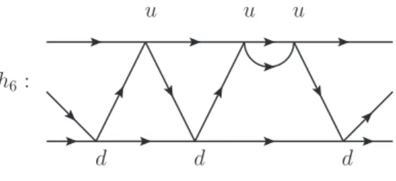
A hooked 3-lines hq with q hooks consists of 3 lines, the upper line, the middle line and the lower line, such that the middle line moves in a zigzag between the upper line and the lower line forming q hooks labeled byu (a hook formed by the upper line and the middle line) or d (a hook formed by the lower line and middle line) as shown below as an example in Figure 2.
As a special case of a hooked 3-lines diagram, we have a truss bridge diagram:
Definition 2.2. A hooked 3-lines diagram generated by the sequenceudud . . . ud or udud . . . udu is called a “truss bridge diagram”. We denote by Tn the truss bridge diagram with n-trusses.
d d d
u u u
h6:
Figure 2. A hooked 3-lines associated with “duduud”.
Figure 3. The truss bride T3 (ududu).
Hereafter, we always assume the following two conditions.
(H1) The space-time dimension is 2, i.e., ν = 2.
(H2) The masses assigned to internal lines are all equal to m >0.
§3. Pinch points and cusps of T1, T2 and T3
We study, in this section, singularity structure of the nonzero-α LN surface L⊗ ⊂ Rνn associated with the truss bridge diagram Tn of lower degree (n = 1,2,3). Here a singular point of L⊗ is, by definition, a point in the (topological) closure [L⊗] of L⊗ at which [L⊗] is not real analytic smooth, and we denote by [L⊗]sing the set of singular points of L⊗. To make its structure easily understood, we present several pictures of [L⊗] drawn by a computer, in which one can observe a specific shape so called a “Whitney umbrella” near [L⊗]sing. As a matter of fact, [L⊗]sing consists of the following two kinds of singularity: Let Ω be an open subset in RdimRL⊗, and let ϕ: Ω→Rνn be a real analytic map such thatϕ(Ω) = [L⊗] and ϕgives an isomorphism between Ω\ϕ−1([L⊗]sing) and [L⊗]\[L⊗]sing. Such an analytic map ϕ is sometimes called parametrization of L⊗.
• A pinch point: the image of a critical point of ϕ. That is, p∈[L⊗] is a pinch point if and only if there exists q ∈ Ω with p = ϕ(q) such that the rank of dϕ becomes less than dimRL⊗ at q.
• A cusp: a self-intersection point of [L⊗]. That is, a point p∈ [L⊗] is called a cusp if and only if there exist distinct points q1 and q2 in Ω with p=ϕ(q1) =ϕ(q2).
Note that subsequent computations are performed with the following conventions.
1. For a vector v = (v0, v1)∈R2, we apply the linear transformation (3.1) ev0 =v0+v1, ev1 =v0−v1
to internal and external vectors. All the computations are performed with the new coordinates.
2. Hence Lorentz metric v2 = v20 − v12 for v = (v0, v1) becomes ev0ve1 in the new coordinates (ev0, ev1).
3. All the masses assigned to internal lines are assumed to be 1.
§3.1. The singularity structure of the nonzero-α LN surface of T1
Let us first consider the truss bridge diagram T1. We have essentially 3-external lines which emanate from the vertices A, B and C, and hence, the dimension of the space of external vectors is 6. However, since the sum of the external vectors must be zero by the energy-momentum conservation laws and since the LN surface is Lorentz invariant, we can regard the nonzero-α LN surface L⊗(T1) as a surface in R3.
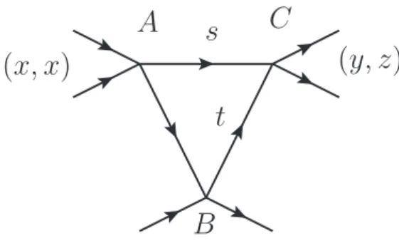
We specify the coordinates (x, y, z) of the external vectors as described in Fig.4, that is, the external vector on the line from A is (x, x) and that from C is (y, z).
( x, x ) ( y, z )
s t A
B
C
Figure 4. The truss bridge diagram T1.
In what follows, for example, the symbolABdenotes not only the lineABitself but also an internal vector on this line. Set AC = (s, 1/s) and BC = (t, 1/t) for positive real numbers s > 0 and t > 0. Then, by the energy-momentum conservation laws at
the vertex A, we obtain AB = (1/s, s). Hence, by using parameters s > 0 and t > 0, each internal vector is expressed by
(3.2) AB = (1/s, s), AC = (s, 1/s), BC = (t, 1/t), and we define the analytic map ϕ:R2>0 →R3 by
(3.3)
x=s+ 1/s, y=s+t, z = 1/s+ 1/t.
The map ϕgives the required parametrization of L⊗(T1) as we will see.
We first compute a pinch point of T1. Note that we have
(3.4) dx= (1−1/s2)ds, dy =ds+dt, dz=−1/s2ds−1/t2dt.
If s 6= 1, clearly we get dx∧dy 6= 0. Furthermore, when s = 1 and t 6= 1, we have dy∧dz 6= 0. Therefore dϕ degenerates only ats =t= 1, and hence, the pinch point of T1 is just one point given by
(3.5) (s, t) = (1, 1), that is, (x, y, z) = (2, 2, 2).
Remark 3.1. We have the equivalence
(3.6) (s, t) = (1, 1) ⇐⇒ AB =AC =BC.
Hence we can conclude that the external vectors are located at a pinch point ofT1 when all the internal vectors coincide.
Now let us compute cusps of T1. It suffices to determine points where ϕ is not injective. Note
(3.7)
x=s+ 1/s, y=s+t, z = 1/s+ 1/t,
⇐⇒
s x−s2 −1 = 0, y−t−s = 0, s t z−t−s= 0.
Suppose that (s1, t1) and (s2, t2) give the same x,y andz. Then we may assume either s1 6=s2 or t1 6= t2. We first consider the case t1 6= t2. By eliminating the variable s of the first and the second equations in (3.7), we obtain
−t2+ (2y−x)t−y2+x y−1 = 0,
and, by the first and the third ones in (3.7), we have (−z2+x z−1)
t2+ (2z −x) t−1 = 0.
Then, as both the equations share two rootst1andt2, by employing Euclidean algorithm (in this case, it is enough to divide the first equation by the second one and get its remainder since the second equation is of the second order), we have, for any t,
((−2y+x) z2+(
2x y−x2+ 2)
z −2y) ( t+
y2−x y+ 1)
z2+(
−x y2+x2y−x)
z+y2−x y = 0, that is, {
(−2y+x) z2+(
2x y−x2+ 2)
z−2y = 0, (y2−x y+ 1)
z2+(
−x y2+x2y−x)
z+y2−x y = 0.
By putting (3.3) into these equations, we have
(s−1) (s+ 1) (t+s) (s t−1)
s2t2 = 0,
(s−1) (s+ 1) (t+s) (s t−1)
s2t = 0.
Therefore either s = 1 or st = 1 holds. Suppose s = 1. Then we have x = 2, and thus, we get s1 = s2 = 1, which contradicts t1 =6 t2 because of y−t−s = 0 in (3.7).
Hence we exclude s = 1. On the other hand, on {st = 1}, ϕ is not injective because (s, t) = (s∗, 1/s∗) and (s, t) = (1/s∗, s∗) give the same (x, y, z). By applying the same argument to the case s1 6=s2, we obtain the same set {st= 1} on which ϕis not injective.
Summing up,ϕ is injective on {st6= 1}, that is, the restriction (3.8) ϕ:R2>0\ {st= 1} →R3
becomes an embedding. Furthermore, the image of {st = 1} by ϕ is the half line {x=y =z}withx≥2, and it is doubly covered byϕ. Hence the cusps ofL⊗(T1) form an open half line
(3.9) {(x, y, z)∈R3; x=y =z, x >2} whose end-point is the pinch point (2, 2,2).
Remark 3.2. As a pinch point is characterized by a configuration of internal vec- tors, we can also characterize cusps in terms of a configuration of the internal vectors.
Since we have
(3.10) st= 1 ⇐⇒ AB =BC,
the external vectors are located at a cusp when the internal vectorsABandBC coincide.
2
2.1
2.2
2.3
2.4
2.5
2.6
2.7
2.8
2.9 X axis
1 1.5 2
2.5 3
3.5 4
Y axis 1
1.5 2 2.5 3 3.5 4 4.5 5
Z axis
Figure 5. L⊗(T1) viewed from (116,287).
2 2.1
2.2 2.3
2.4 2.5
2.6 2.7
2.8 2.9
X axis
1 1.5 2 2.5 3 3.5
4 Y axis
1
1.5
2
2.5
3
3.5
4
4.5
5 Z axis
Figure 6. L⊗(T1) viewed from (281,289).
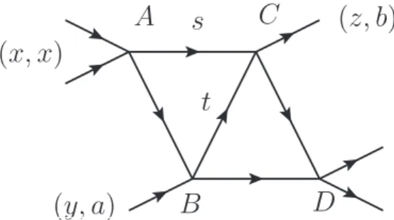
§3.2. The singularity structure of the nonzero-α LN surface of T2 Let us consider the truss bridge diagram T2. We have essentially 4-external lines which emanate from the vertices A, B, C and D, and hence, the dimension of the space of external vectors is 8. By the same reasoning as that in T1, we can regard the nonzero-α LN surface L⊗(T2) ofT2 as a hypersurface in R5. However the dimension of the ambient space is still too big to understand L⊗(T2) visually. Therefore, instead of studying the hypersurface inR5directly, we consider a family of slices ofL⊗(T2) cut with 3-dimensional linear subspaces, where we choose each subspace so that it transversally intersects with the singular points of L⊗(T2).
Let a and b be real numbers. Then we specify the coordinates (x, y, z) and the parameters (a, b) of the external vectors as described in Fig.7, that is, the external vector on the line from A is (x, x), that from B is (y, a) and that from C is (z, b).
( x, x )
( y, a )
( z, b ) s
t A
B
C
D
Figure 7. The truss bridge diagram T2.
Let s and t be positive real numbers. We set
(3.11) AC = (s, 1/s), BC = (t, 1/t).
Then, by considering the energy-momentum conservation laws at each vertexA,B and C, we obtain
(3.12)
AB = (1/s, s), AC = (s, 1/s), BC = (t, 1/t), BD =
( t
s t+a t−1, s t+a t−1 t
) , CD =
(
− s t
b s t−t−s, −b s t−t−s s t
) .
Note that, since an internal vector is located in the future light cone, i.e., the region {(v0, v1); v0 >0, v1 >0}, (s, t) belongs to
(3.13) Ω :={(s, t)∈R2>0; st+at−1>0, t+s−bst > 0}.
Then the real analytic map ϕ: Ω→R3 is defined by
(3.14)
x=s+ 1/s,
y= s2t2+a s t2−s t−a t+ 1 s (s t+a t−1) , z = b s t2−t2+b s2t−s t−s2
b s t−t−s .
This ϕgives the required parametrization of a slice of L⊗(T2). Note that the slice is a surface in R3 and it is also called the nonzero-α LN surface for simplicity.
We can compute pinch points and cusps by the same arguments as those for T1. The pinch points ofT2 are the following 3-points:
(P1) (s, t) = (1, 1), i.e.,
(3.15) (x, y, z) =
( 2, 1
a, 2b−3 b−2
) .
The external vectors are located at this pinch point if and only if the configuration of internal vectors becomes
(3.16) AB =BC =AC.
(P2) (s, t) = (1
b, 2b ab+ 1
) , i.e.,
(3.17) (x, y, z) =
(b2+ 1
b , −b (a b−3) a b+ 1 , 1
b )
.
The external vectors are located at this pinch point if and only if the configuration of internal vectors becomes
(3.18) BC =CD =BD.
(P3) (s, t) = (
1, 2 a+b
) , i.e.,
(3.19) (x, y, z) = (
2, −b2−2b−a2+ 2a+ 4
(b−a−2) (b+a) , b2+ 2b−a2−2a−4 (b−a−2) (b+a)
) . The external vectors are located at this pinch point if and only if the configuration of internal vectors becomes
(3.20) AB =AC, BD =CD.
The cusps of T2 are given as follows. Note that, outside these cusps, ϕ becomes an embedding.
(C1) The image of {st= 1}, which is the half curve defined by (3.21) (x−z)(x−b) = 1, y= 1/a (x > 2).
Note that its end-point is the pinch point (P1). Furthermore, this half curve is realized by the configuration of internal vectors with
(3.22) AB =BC.
(C2) The image of {s = 1/b}, which is the half line defined by (3.23) x= b2+ 1
b , z = 1/b
(
y > −b (a b−3) a b+ 1
) .
Note that its end-point is the pinch point (P2). This half line is realized by the configuration of internal vectors with
(3.24) BC =CD.
(C3) This is a half portion of some analytic curve C whose end-point is the pinch point (P3). The defining equation ofC is very complicated and long. See also the following remarks.
Remark 3.3. The cusps (C3) is the image by ϕ of the subset in the (s, t)-space
(3.25)
{(b+a) s (s+a) (b s−1) t4 + (s+a) (b s−1) (
b s2+a s2−2s−b−a) t3
−(s−1) (s+ 1) (
2b s2+a s2+b2s+ 3a b s+a2s−2s−b−2a) t2 + (s−1) (s+ 1) (
s2+ 2b s+ 2a s−1)
t+s (
1−s2)
= 0} .
Remark 3.4. Clear description of a configuration of internal vectors which realizes a point in the cusps (C3) is not yet known. For a specific (a, b), however, we have simple description of these cusps as follows: Suppose a = b. Then we can easily confirm that the distinct points
(s, t) = (s∗, 1/a) and (s, t) = (1/s∗, 1/a) (s∗ >0, s∗ 6= 1) give the same (x, y, z) by ϕ. The image of these points is defined by
(3.26) y =z = 1/a (x >2),
and it is the cusps (C3) when a =b.
Furthermore, when a is sufficiently close to b, we can find the cusps (C3) in the following way: Set s=s(x) := 2−1(x+√
x2−4) (x >2) and
(3.27)
F(ρ, σ; x, a, b) :=
(
ρ+ 1
s+a−ρ−1 −s−1 )
− (
σ+ 1
s−1+a−σ−1 −s )
, G(ρ, σ; x, a, b) :=
(
s+ρ− 1
s−1+ρ−1−b )
− (
s−1+σ− 1 s+σ−1−b
) . Define the subspace H ⊂R5 by
(3.28) {(ρ, σ, x, a, b)∈R5; a =b, ρ=σ =a−1}. We can easily confirm
(3.29) F|H =G|H = 0.
Since
(3.30) ∂ρF|H = 1−a2s−2, ∂σF|H =−1 +a2s2,
∂ρG|H = 1−a2s2, ∂σG|H =−1 +a2s−2 hold, we get
(3.31) J|H = det (
∂ρF ∂σF
∂ρG ∂σG )
H
= 2a2(s−2−s2) +a4(s4−s−4).
Then, by noticing
(3.32) s2−s−2 =x(s−s−1), s4−s−4 =x(x2−2)(s−s−1), we have
(3.33) J|H =a2x(s−s−1)(a2(x2−2)−2), from which J|H 6= 0 follows if x > 2 and x 6= √
2/a2+ 2. Hence we can find an open subset D in {(x, a, b)∈ R3;x >2} such that it is an open neighborhood of the locally closed subset
(3.34) {(x, a, b)∈R3;x > 2, x6=√
2/a2+ 2, a=b}
and there exist real analytic functions ρ = ρ(x;a, b) and σ = σ(x;a, b) defined on D satisfying
(3.35)
F(ρ(x;a, b), σ(x;a, b); x, a, b) = 0 ((x, a, b)∈D), G(ρ(x;a, b), σ(x;a, b); x, a, b) = 0 ((x, a, b)∈D), ρ(x;a, a) =σ(x;a, a) = 1/a ((x, a, a)∈D).
Now define 2-points
(3.36) q1 = (s∗, ρ(x∗;a, b)), q2 = (1/s∗, σ(x∗;a, b)),
where x∗ :=s∗ + 1/s∗ and s∗ is a positive real number satisfying (x∗, a, b)∈ D. Then, since ρ and σ satisfy F = G = 0, the points q1 and q2 give the same (x, y, z) by ϕ.
The (x, y, z) thus obtained belongs to the cusps (C3) because q1 6=q2 and ρ(x;a, a) = σ(x;a, a) = 1/a hold.
2 2.002 2.004 2.006 X axis 2.008 2.01 2.65
2.7 2.75 2.8 2.85 2.9 2.95 3 3.05 Y axis (x2) 1.02
1.04 1.06 1.08 1.1 1.12 1.14
Z axis
Figure 8. L⊗(T2) with (a, b) = (0.7, 0.95) viewed from (90,320).
2 2.002
2.004 2.006
2.008 2.01
X axis 3.05 3 2.95 2.9 2.85Y axis (x2) 2.8 2.75 2.7 2.65
1.02
1.04
1.06
1.08
1.1
1.12
1.14 Z axis
Figure 9. L⊗(T2) with (a, b) = (0.7, 0.95) viewed from (281,291).
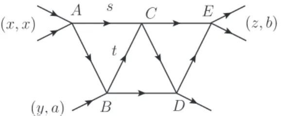
§3.3. The singularity structure of the LN surface of T3
Let us now consider the truss bridge diagram T3. By the same reasoning as that for T2, the nonzero-α LN surface L⊗(T3) of T3 can be regarded as a subset in R5, and hence, we need to consider a family of slices of L⊗(T3) cut with 3-dimensional linear subspaces. Let a and bbe real numbers. Then we specify the coordinates (x, y, z) and the parameters (a, b) of the external vectors in the same way as that for T2 (see Fig.10 also).
(x, x)
(y, a)
(z, b) s
t A
B C
D E
Figure 10. The truss bridge diagram T3.
The biggest difference betweenT2 and T3 is existence of the “non-external vertex”
C, that strongly constrains a configuration of internal vectors. As a matter of fact, it follows from Lemma 3.2 [5] that internal vectors satisfy either (A) or (B) below:
(3.37) (A) AC =CD and BC =CE (B) AC =CE and BC =CD.
Therefore we have a different component of L⊗(T3) corresponding to either (A) or (B).
3.3.1. The component of L⊗(T3) with the configuration (A)
We first study the component of L⊗(T3) where internal vectors satisfy the config- uration (A). Note that, in this case, each slice of the component becomes a surface.
Set
(3.38) AC = (s, 1/s) and BC = (t, 1/t).
Then, it follows from the energy-momentum conservation laws and the configuration (A) that we have
(3.39)
AC =CD= (s, 1/s), AB = (1/s, s), BC =CE = (t, 1/t), BD =
( t
s t+a t−1, s t+a t−1 t
) , DE =
( t
b t−1, b t−1 t
) .
Define
Ω :={(s, t)∈R2>0; bt−1>0, st+at−1>0}, and the analytic map ϕ: Ω→R3 by
(3.40)
x=s+ 1/s,
y= s2t2+a s t2−s t−a t+ 1 s (s t+a t−1) , z = b t2
b t−1.
This ϕ gives the required parametrization of a slice of the component of L⊗(T3) with the configuration (A). The slice becomes a surface in the 3-dimensional linear space and it is often called the “surface component” of T3.
The pinch points are the following 3-points:
(P1) (s, t) = (
1, 1 a
) , i.e.,
(3.41) (x, y, z) =
(
2, 1/a, b a (b−a)
) .
The external vectors are located at this pinch point if and only if the configuration of internal vectors becomes
(3.42) AB =BD =AC (=CD).
(P2) (s, t) = (
b−a, 2 b
) , i.e.,
(3.43) (x, y, z) =
(
b−a+ 1
b−a, 3b−4a b(b−a),4/b
) .
The external vectors are located at this pinch point if and only if the configuration of internal vectors becomes
(3.44) (BC =) CE =BD =DE.
(P3) (s, t) = (
1, 2 b
) , i.e., (3.45) (x, y, z) =
(
2, −b2−2a b−2b+ 4a+ 4 b (b−2a−2) , 4/b
) .
The external vectors are located at this pinch point if and only if the configuration of internal vectors becomes
(3.46) (CD =) AC =AB, (BC =) CE =DE.
The cusps of T3 are given as follows. Note that, outside these cusps, ϕ becomes an embedding.
(C1) The image of {t = 1/a}, which is the half line defined by
(3.47) y= 1
a, z = b
a (b−a) (x >2).
Note that its end-point is the pinch point (P1). Furthermore, this half line is realized by the configuration of internal vectors with
(3.48) AB =BD.
(C2) The image of {s =b−a}, which is the half line defined by
(3.49) x =b−a+ 1
b−a, y=z− 1
b−a (z >4/b).
Note that its end-point is the pinch point (P2). Furthermore, this half line is realized by the configuration of internal vectors with
(3.50) BD =DE.
(C3) This is a half portion of some analytic curve C whose end-point is the pinch point (P3). The defining equation of C is very complicated and long. See also Remark 3.5 below. The situation is quite similar to the one for the cusps (C3) of T2.
Remark 3.5. The cusps (C3) is the image by ϕ of the subset in the (s, t)-space
(3.51)
{b s (s+a) (b s−a s−1) t4 + (s+a) (b s−a s−1) (
b s2−2s−b) t3
−(s−1) (s+ 1) (
2b s2−a s2+b2s+a b s−a2s−2s−b−a) t2 + (s−1) (s+ 1) (
s2+ 2b s−1)
t+s (
1−s2)
= 0} .
2
2.001
2.002
2.003
2.004
2.005 X axis
2.19 2.2 2.21 2.22 2.23 2.24 2.25 2.26 2.27 2.28
Y axis (x2) 2.055
2.06 2.065 2.07 2.075
Z axis
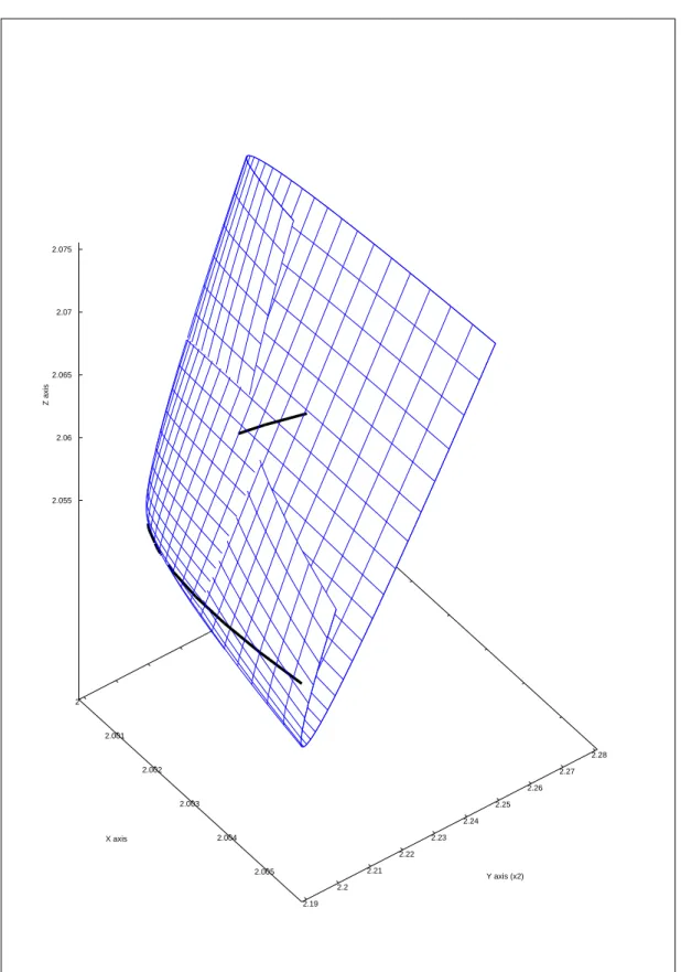
Figure 11. L⊗(T3) with (A) and (a, b) = (0.9, 1.95) viewed from (119,306).
2 2.001 2.002 2.003 2.004 2.005
X axis 2.19
2.2 2.21 2.22
2.23 2.24
2.25 2.26
2.27 2.28 Y axis (x2)
2.055 2.06 2.065 2.07 2.075
Z axis
Figure 12. L⊗(T3) with (A) and (a, b) = (0.9, 1.95) viewed from (119,306).
3.3.2. The component of L⊗(T3) with the configuration (B)
We now study the component of L⊗(T3) where internal vectors satisfy the config- uration (B). Note that, in this case, each slice of the component becomes a curve in the 3-dimensional linear space and it is often called the “non-surface component” or the
“higher codimensional component”.
Lets > 0, and we setAC = (s, 1/s). It follows from the configuration (B) and the closed loop condition for the triangle 4BCD that the internal vectors satisfy
(3.52) AC =CE, BC =BD =CD.
Then, the internal vectors are uniquely determined by the condition (3.52) and the energy-momentum conservation laws at each vertex as follows.
(3.53)
AC =CE = (s, 1/s), AB = (1/s, s), BC =CD =BD=
( 2
s+a, s+a 2
) , DE=
( s
b s−1, b s−1 s
) .
Remark 3.6. When a Feynman graph has a non-external vertex, generally speak- ing, its nonzero-α LN surface may have a higher codimensional component.
Define
(3.54) Ω ={s∈R>0; s+a > 0, bs−1>0}, and the analytic map ϕ: Ω→R3 by
(3.55)
x=s+ 1/s, y= 3s−a
s (s+a), z = b s2
b s−1.
Then the mapϕgives the required parametrization of the higher codimensional compo- nent ofT3. Note that this curve is smooth if (a, b)6= (1, 2), and it has only one singular point s= 1, i.e., (x, y, z) = (2, 2, 2) if (a, b) = (1, 2).
2
2.001
2.002
2.003
2.004
2.005
2.19 2.2 2.21 2.22 2.23 2.24 2.25 2.26 2.27 2.28 2.055
2.06 2.065 2.07 2.075
Figure 13. L⊗(T3) with (B) and (a, b) = (0.9, 1.95): The curve which crosses the surface is the non-surface component, viewed from (119,306).
2 2.001 2.002 2.003 2.004 2.005
2.19 2.2 2.21 2.22 2.23 2.24 2.25 2.26 2.27 2.28
2.055 2.06 2.065 2.07 2.075
Figure 14. L⊗(T3) with (B) and (a, b) = (0.9, 1.95): The curve which crosses the surface is the non-surface component, viewed from (119,306).
§4. An acnode in the Landau-Nakanishi geometry of T2
An acnode (i.e., an isolated point) appearing in the Landau-Nakanishi geometry of T2 was first found by R. J. Eden et al. [1] (see also [2]). We study, in this section, its origin from the viewpoint of singularity structure.
(b) (c) (d)
Figure 15. A rough picture of acnodes described in p.106 [2].
In the book [2], R. J. Eden et al. had studied a family ofLN curves ofT2, which is, by definition, the intersection of L⊕(T2) and a parameterized family of 2-dimensional subspaces. They first change a parameter of the family to the complex domain, and then, put it back to the real domain. After these changes of a parameter, they found an isolated point (acnode) apart from the curve as it is shown in Fig.15. By further continuous changes of a parameter (from (b) to (d) in Fig.15), the acnode continuously moves and finally disappears after it hits on the curve.
2
2.1
2.2
2.3
2.4
2.5
2.6
2.7
2.8
2.9 X axis
1 1.5 2 2.5 3 3.5 4
Y axis 1
1.5 2 2.5 3 3.5 4 4.5 5
Z axis
Figure 16. L⊗(T1).
1.6
1.8
2
2.2
2.4
2.6
2.8
1 1.5 2 2.5 3 3.5 4 1 1.5 2 2.5 3 3.5 4 4.5 5
Figure 17. The analytic closure of L⊗(T1).
At first glance, existence of such an acnode seems strange because the nonzero-α LN surface of T2 generically has a shape like the one drawn in Fig.8, and thus, it is impossible to obtain an isolated point possessed with such a behavior when we cut the surface with a suitable family of 2-dimensional subspaces in R3. Singularity structure studied in the previous section, however, can explain an origin of the acnode. In fact, the cusps in T1, T2 and T3 are half portions of real analytic curves. Hence, if we take the analytic closures of these surfaces, the whole parts of these curves appear. For example, if we take the analytic closure of the nonzero-α LN surface of T1, then we get the original surface with the whole line and a half portion of this line is located far from the surface as Fig.17 shows.
Furthermore, their change of a parameter to the complex domain entails complexifi- cation of the nonzero-α LN surface ofT2. As a consequence, when they put a parameter back to the real domain, the resulting surface contains the analytic closure of the origi- nal surface. Hence the acnode they observed can be understood as a point in a portion of an analytic extension of some cusps which is located far from the surface itself.
We give, in Fig.18, some slices of the analytic closure of the nonzero-α LN surface of T2 cut with the 2-dimensional linear subspace {(x, y, z)∈R3; x+y= k}. One can surely find an isolated point (acnode) which continuously moves and disappears after it hits on the curve. We note that, if we consider a region which is much wider than that shown below, we find another acnode as in Fig.15 (b) (see Fig. 19).
Figure 18. Slices by {x+y=k}.
0.8 0.85 0.9 0.95 1 1.05 1.1 1.15 1.2 1.25 1.3
1.86 1.88 1.9 1.92 1.94 1.96 1.98 2 2.02 2.04
Figure 19. Slices by {x+y= 3.32} in the wider region.
§5. The non-surface component of T3
As we pointed out in [3] (see Section 3 of this article also), L⊕(T3) contains two components; one a hypersurface and the other with codimension 2. This is a phe- nomenon which is not observed in L⊕(G) ifGhas no non-external vertex. In [3] and [5]
we studied the non-surface component (i.e., the codimension 2 component) of L⊕(T3) by using the property that it coincides with the intersection of twoLN surfaces associ- ated with ice-cream cone diagrams IL and IR, which are obtained by contracting some parts of T3 ([5, Section 5]). Here we present another approach that we understand the non-surface component from the viewpoint of singularity structure of a surface compo- nent. We first introduce the complemented truss bridge diagram Te3 by adding an extra external line to the non-external vertex of T3 and compute its pinch points and cusps.
Then we investigate correspondence between the non-surface component of T3 and the restriction of pinch points and cusps of Te3 to the ambient space of T3.
§5.1. The complemented truss bridge diagram Te3
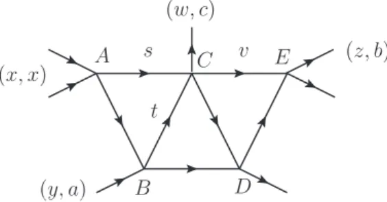
The complemented truss bridge diagramTe3is described in Fig. 20, which is obtained by addition of the external line to the vertexC ofT3. It has 5-external lines, and hence, the nonzero-α LN surfaceL⊗(Te3) ofTe3 is regarded as a hypersurface inR7. In this case, we consider a family of slices of L⊗(Te3) cut with 4-dimensional linear subspaces. Let a, band cbe real numbers. We specify the coordinates (x, y, z, w) and the parameters (a, b, c) of the external vectors as described in Fig.20, that is, the external vector on the line from A is (x, x), that from B is (y, a), that from C is (w, c) and that from E is (z, b). Note that the ambient space of T3 is identified with the subspace {w =c= 0} in this situation.
(w, c) (x, x)
(y, a)
(z, b) s
t A v
B C
D E
Figure 20. The complemented truss bridge diagram Te3.
Remark 5.1. The reason why we consider slices cut with 4-dimensional subspaces instead of 3-dimensional ones is as follows: As we will see later, there exists a connected component of pinch points ofTe3 which has non-transversal intersection with the ambient
space of T3, i.e., the subspace {w = c = 0}. Hence we need, at least, a 4-dimensional linear subspace so that it contains the ambient space ofT3and it intersects transversally with each component of singular points ofTe3.
Let s, t and v be positive real numbers, and set
(5.1) AC = (s, 1/s), BC = (t, 1/t), CE = (v, 1/v).
Then it follows from the energy-momentum conservation laws that the internal vectors are given by
(5.2)
AC = (s, 1/s), AB = (1/s, s), BC = (t, 1/t), CE = (v, 1/v), CD =
(
− s t v
c s t v−t v−s v+s t, −c s t v−t v−s v+s t s t v
) , BD =
( t
s t+a t−1, s t+a t−1 t
) , DE =
( v
b v−1, b v−1 v
) . Set
(5.3) Ω :={(s, t, v)∈R3>0; bv−1>0, st+at−1>0, −cstv+tv+sv−st >0}. Then the analytic map ϕ: Ω→R4 is defined by
(5.4)
x=s+ 1/s,
y= s2t2+a s t2−s t−a t+ 1 s (s t+a t−1) , z = b v2
b v−1,
w=−c s t v2−t v2−s v2−c s t2v+t2v−c s2t v+ 2s t v+s2v−s t2−s2t
c s t v−t v−s v+s t .
This ϕ gives parametrization of a slice of L⊗(Te3).
§5.2. Pinch points of the complemented truss bridge diagram Te3
Let us compute dϕ. Since x (resp. z) depends only on s (resp. v) and y depends only on s and t, the 3×4 Jacobian matrix ofϕ takes a form as
(5.5) J :=
∂x
∂s 0 ∂y
∂s
∂w
∂s 0 ∂z
∂v 0 ∂w
∂v 0 0 ∂y
∂t
∂w
∂t
.
We also have
(5.6) ∂x
∂s = (s−1) (s+ 1)
s2 , ∂z
∂v = b v (b v−2) (b v−1)2 , from which
(5.7) ∂x
∂s = 0 ⇐⇒ s = 1 and ∂z
∂v = 0 ⇐⇒ v= 2/b
follows. By taking these observations into account, we compute a pinch point at which Rank(J)<3 holds.
Case I: s 6= 1 andv 6= 2/b.
In this case, we have
Rank(J)<3 ⇐⇒ ∂y
∂t = 0 and ∂w
∂t = 0.
Since
∂y
∂t = (s+a) t (s t+a t−2) (s t+a t−1)2
and ∂w
∂t = t (c s v−v+s) (c s t v−t v−2s v+s t) (c s t v−t v−s v+s t)2
hold, we conclude that Rank(J)<3 if and only if { (s t+a t−2) = 0,
(c s v−v+s) = 0.
Here we use the facts s+ a > 0 and −cstv + tv + 2sv − st > 0 which follow from the conditions st+at−1 > 0 and −cstv +tv +sv−st > 0. Summing up, we have one component of pinch points: Here we note that we find CD = −BD by (5.2) if cstv−tv−2sv+st= 0 and hence the point in question is located outside the region of our concern in this paper.
(I.a) t= 2
s+a and v=− s
c s−1 (s free). For these parameters, we have
(5.8) w= c s2
c s−1.
We can understand the pinch points (I.a) through a configuration of internal vec- tors. First note that
(5.9) t = 2
s+a ⇐⇒ BC =BD and v=− s
c s−1 ⇐⇒ BC =CD.
Therefore the external vectors are located at a pinch point (I.a) if and only if the configuration of internal vectors satisfy
(5.10) BC =BD =CD.
In particular, when c= 0, we have w= 0 by (5.8) which implies v=s, i.e.,AC =CE.
Summing up, if c= 0, we get
(5.11) BC =BD =CD, AC =CE,
and thus, it follows from (3.52) that the restriction of pinch points (I.a) to {w =c= 0} coincides with the non-surface component of T3.
Case II: s= 1 and v6= 2/b.
In this case,
Rank(J)<3 ⇐⇒ ∂y
∂s
∂w
∂t − ∂y
∂t
∂w
∂s = 0.
As we have (∂y
∂s
∂w
∂t − ∂y
∂t
∂w
∂s )
s=1
=−(t−1) t (t+ 1) (c v−a v−2v+ 1) (c t v+a t v−2v+t) (a t+t−1)2(c t v−t v−v+t)2 , we obtain 3-components of pinch points:
(II.a) s= 1 and t = 1 (v free). For these parameters, we have (5.12) w=−c v2−2v2−2c v+ 4v−2
c v−2v+ 1 and, in particular, when c= 0,
(5.13) w =−2 (v−1)2
2v−1 holds.
(II.b) s = 1 and v=− 1
c−a−2 (t free). For these parameters, we have
(5.14) w = a c t2+c t2−a2t2−3a t2−2t2+a c t+c t−a2t−2a t−t−c+a+ 1 (c−a−2) (a t+t−1)
and, in particular, when c= 0,
(5.15) w= (a+ 1) (t+ 1) (a t+ 2t−1) (a+ 2) (a t+t−1) .
In this case, (5.2) entails CD = −BD; hence the point in question is located outside the region of our concern in this paper.
(II.c) s = 1 andv =− t
(c+a) t−2 (t free). For these parameters, we have (5.16)
w= a c t3+c t3+a2t3+a t3+a c t2−c t2+a2t2−2a t2−t2−c t−3a t+t+ 2 (a t+t−1) (c t+a t−2)
and, in particular, when c= 0,
(5.17) w = (t+ 1) (a t−1) (a t+t−2) (a t−2) (a t+t−1) .
Note that this component passes through a pinch point of T3 when t = 1/a and it also intersects with the non-surface component of T3 when t= 2/(a+ 1).
Case III: s6= 1 and v= 2/b.
In this case,
Rank(J)<3 ⇐⇒ ∂y
∂t
∂w
∂v = 0.
By noticing
∂y
∂t
∂w
∂v
v=2/b
= 4 (s+a) t (s t+a t−2) (c s t−t−s) (c s t+b s t−t−s) (s t+a t−1)2(2c s t+b s t−2t−2s)2 , we have 3-components of pinch points:
(III.a) v = 2/band t = 2
s+a (s free). For these parameters, we have (5.18)
w =(
b s4−2b c s3−b2s3+ 2a b s3−2s3−2a b c s2+ 4c s2−a b2s2+a2b s2 + 4b s2−4a s2−4b c s+ 4a c s−2b2s+ 4a b s−2a2s−4s+ 4b−4a) / (
b(s+a) (
s2−2c s−b s+a s+ 2) ) and, in particular, when c= 0,
(5.19) w= (s−b+a) (b s−2) (
s2+a s+ 2) b (s+a) (s2−b s+a s+ 2) .
Note that this component passes through a pinch point of T3 whens=b−a and it also intersects with the non-surface component of T3 when s= 2/b.
(III.b) v= 2/b and t= s
c s−1 (s free). For these parameters, we have
(5.20) w= c s2
c s−1.
In this case, (5.2) entails CD = −CE, and hence, the point in question is located outside the region of our concern in this paper.
(III.c) v= 2/band t = s
(c+b) s−1 (s free). For these parameters, we have (5.21) w = b c s2+b2s2−4c s−4b s+ 4
b (c s+b s−1) and, in particular, when c= 0,
(5.22) w= (b s−2)2
b (b s−1).
Case IV: s= 1 and v= 2/b.
Always Rank(J)<3 in this case. Hence we have one component of pinch points:
(IV.a) s = 1 andv = 2/b(t free). For these parameters, we have
(5.23) w = 2b c t2+b2t2−2b t2+ 2b c t−4c t+b2t−4b t+ 4t−2b+ 4 b (2c t+b t−2t−2)
and, in particular, when c= 0,
(5.24) w= (b−2) (t+ 1) (b t−2) b (b t−2t−2) .
Note that this component passes through a pinch point of T3 when t= 2/b.
Summing up, for the restriction of pinch points ofTe3to the ambient space ofT3, i.e., the subspace{w=c= 0}, we have observed the following two facts: The 3-components (II.c), (III.a) and (IV.a) of pinch points of Te3 transversally intersect with the ambient space of T3 for generic parameters. Their intersection contains all pinch points of T3.
The component (I.a) of pinch points ofTe3, however, has non-transversal intersection with the ambient space of T3. The important fact is that their intersection is nothing but the non-surface component of T3.
![Figure 15. A rough picture of acnodes described in p.106 [2].](https://thumb-ap.123doks.com/thumbv2/123deta/5796002.1529809/26.892.192.710.295.436/figure-rough-picture-acnodes-described-p.webp)