Anal ys i s of ec onom
i c pot ent i al s of
i nf r as t r uc t ur e devel opm
ent s i n and ar ound
Bhut an
著者
Kum
agai Sat or u, I s ono I kum
o, Kenm
ei Ts ubot a
権利
Copyr i ght s 日本貿易振興機構(ジェトロ)アジア
経済研究所 / I ns t i t ut e of D
evel opi ng
Ec onom
i es , J apan Ext er nal Tr ade O
r gani z at i on
( I D
E- J ETRO
) ht t p: / / w
w
w
. i de. go. j p
j our nal or
publ i c at i on t i t l e
I D
E D
i s c us s i on Paper
vol um
e
702
year
2018- 03
INSTITUTE OF DEVELOPING ECONOMIES
IDE Discussion Papers are preliminary materials circulated to stimulate discussions and critical comments
Keywords: Simulation, new economic geography, Bhutan JEL classification: R12, R13, R42
1 Director, Economic Geography Study Group, Development Studies Center, IDE-JETRO ([email protected])
IDE DISCUSSION PAPER No. 702
Analysis of Economic Potentials of
Infrastructure Developments in and
around Bhutan
Satoru Kumagai
1, Ikumo ISONO
2and
Kenmei TSUBOTA
3March 2018
Abstract
2 Overseas Research Fellow (Sevilla), IDE-JETRO ([email protected])
3 Corresponding author. Research fellow, IDE-JETRO([email protected])
The Institute of Developing Economies (IDE) is a semigovernmental, nonpartisan, nonprofit research institute, founded in 1958. The Institute merged with the Japan External Trade Organization (JETRO) on July 1, 1998.
The Institute conducts basic and comprehensive studies on economic and related affairs in all developing countries and regions, including Asia, the Middle East, Africa, Latin America, Oceania, and Eastern Europe.
The views expressed in this publication are those of the author(s). Publication does not imply endorsement by the Institute of Developing Economies of any of the views expressed within.
INSTITUTE OF DEVELOPING ECONOMIES (IDE), JETRO 3-2-2, WAKABA,MIHAMA-KU,CHIBA-SHI
CHIBA 261-8545, JAPAN
©2018 by Institute of Developing Economies, JETRO
No part of this publication may be reproduced without the prior permission of the
Analysis of Economic Potentials of
Infrastructure Developments
in and around Bhutan
*Satoru Kumagai, Ikumo Isono, and, Kenmei Tsubota
+Institute of Developing Economies, Japan External Trade Organization
March, 2018
This paper conducts a simulation analysis of a spatial economic model in Southern Asia, with a particular focus on Bhutan. It indicates the potential impacts of different infrastructure investments on regional economies in Bhutan and the neighboring countries. The results reveal that road infrastructure investments within Bhutan will likely increase regional accessibility, reshape the monocentric structure of the economy, and induce migration, thereby increasing the real wage for most of Bhutan’s regions. Furthermore, road infrastructure investments within India have some spillover effects on Bhutan, which can be magnified by further reduction in non-tariff barriers.
* We are grateful for the comments and suggestions from Diep Nguyen-Van Houtte and Charles
Kunaka. The findings, interpretations, and conclusions expressed in this work do not necessarily reflect the views of any authorities.
1. Introduction
Some regions benefit from its geographical characteristics and affluent natural resources, considered to be first nature, whereas other regions benefit from the concentration of economic activities and population, considered to be second nature (Krugman 1991). However, landlocked countries and regions may be conceived as inherently lagging behind. Bhutan is one such country, similar to India’s northeastern regions.
This paper considers how possible logistical improvements can potentially enhance the economic activities in such landlocked regions, with particular focus on Bhutan at a regional level but not at a national level. Specifically, we have evaluated the scenarios in line with Bhutan’s 11th five-year plan (2013–2018); its Road Sector Master Plan 2007–2027 (RSMP); and the plans by United Nations Economic and Social Commission for Asia and the Pacific (UNESCAP), South Asian Association for Regional Cooperation (SAARC), and the World Bank. All the projects are supposed to be the “new response and approaches toward achieving long-term development objectives, including the overarching goal of gross national happiness (GNH).”1 In addition, we have examined the road infrastructure project in West Bengal that connects from Kolkata to Bhutan within India’s national development plans. This is because Bhutan’s trade with India constitutes 75.1% of imports and 82.4% of exports. The impacts of such infrastructure projects may or may not be negligible. This road link is crucial to Bhutan as well as northeastern India, as this road is the gateway to the northeastern regions. All the intranational land trade in favor of northeastern regions should come through a part of this link. Thus, certain impacts for all of these regions are expected with road improvements in West Bengal.
We have employed a spatial computable general equilibrium model based on new economic geography (NEG), called a geographical simulation model. The main feature of this simulation model is the evaluation of possible infrastructure improvements at a subnational level and trade and transport facilitation measures.2 It can also provide the scope of analysis covering urbanization, economic clustering, migration within each country, and modal choice.3 As the model considers the subnational level as small as districts in India, the analysis can indicate the geographical impacts and extent in detail.
1 Quoted from the preface of Gross National Happiness Commission (2009).
2 Possible infrastructure projects include upgradation of highways, introduction of multimodal
systems, port expansions, airport renovations, and others. Non-physical infrastructure projects can also include trade facilitation measures, agreements of transshipments, and other measures. These can be considered as long as they are quantitatively measurable. The uniqueness of our model lies in the possible coverage of policy measures.
3 For the impact evaluation of domestic projects, spatial disaggregation within a country is
The impacts of road development projects—North–South Highway (Asian Highway 48), East–West Highway, and Southeast–West Highway—may be larger once all are implemented. This is because each road project targets different parts of regions within Bhutan and increases accessibility to Bhutan.4 Furthermore, Indian parts of SAARC Corridor 3 (West Bengal Corridor) can benefit Bhutan, and such benefits can be magnified by trade facilitations, domestic road network improvements, or both.
Our results only consider economic factors and do not capture environmental impacts or cultural transformation. Hence, it does not comprehensively capture the notion of GNH, which is employed by the government of Bhutan as the national target. However, it does not restrict our results with regard to identifying some unique features of the impact analysis for landlocked regions, and our analysis can provide some policy implications based on them.
The remainder of the paper is organized as follows. Section 2 overviews the regional centers in Bhutan using a population density map and briefly explains the geographical features and regional structure of Bhutan. Subsequently, we show a list of development projects that have been or will be implemented by the government or international organizations. These projects are the candidates for our analysis in the following section. Section 3 describes the structure of the model based on NEG. Section 4 explains the data and parameters. In Section 5, considering each project or the combination of projects as scenarios, we present the results of the impacts for each scenario. Further, we compare the results to overcome the locational disadvantages. Some concluding remarks follow at the end.
2. Overview of the regions
This section overviews the regional structure and infrastructure projects in Bhutan and the surrounding regions. First, we look at the development of socioeconomic indicators, population distribution, migration flows, and trading locations.
2.1. Regional socioeconomic variables
The socioeconomic development of Bhutan in recent decades has been remarkable. Life expectancy at birth was 32.4 in 1960, 45.0 in 1980, and 67.9 in 2010. Per capita gross national income was US$280 in 1982, US$780 in 2000, and US$2370 in 2015. The gross enrollment ratio for primary education was 46.6 in 1980 and reached 111 in 2012.5
In the northeastern Indian states, the per capita net state domestic product in real terms increased substantially from Rs. 1571 in 1980–81 to Rs. 9472 in 1995–
4 Our evaluation is based on real RGDP, which is the combination of RGDP and the accessibility
measure.
96. Infant mortality rate dropped from 60 per 1000 births in 1991 to 51 in 1997. Literacy rates increased from 7% in 1951 to almost 70% in 2001.6 However, its relative position within India is still very low. Pal et al (2015) and Konwar (2015) revealed that the northeastern Indian regions exhibit a higher multidimensional poverty index and, even within these regions, there are high variations in terms of the dimensions of deprivation. They concluded that transport infrastructure is one of the possible remedies for this situation, which shall be considered in the following section.
Bangladesh has been improving its socioeconomic conditions: infant mortality improved from 176 per 1000 births in 1960 to 31 in 2015, life expectancy at birth improved from 46 in 1960 to 72 in 2014, and per capita gross national income improved from US$160 in 1974 to US$1190 in 2015.7
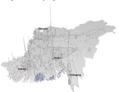
Figure 1. Population Density Map
(a) Population density (Bhutan, Bangladesh and North East India)
6 See Nayak (2009) for details.
(b) Population density (Bhutan, Bangladesh and North East India)
Source: authors’ cartography with LandScan (2010) for population, and GAUL (FAO) for national boundaries.
As mentioned above, all the regions have been growing in the last half of the century in socioeconomic respects. However, their absolute levels are still low and have potential for further improvement. It is quite important to find and implement any measures that alleviate poverty and improve the lives of people in Bhutan. While physical geography of mountainous regions is considered to be a natural obstacle to economic growth, underdeveloped connectivity in plain region has made it even more inaccessible.
The plain region has been historically populous and is still highly populated, as shown in Figure 1(a). With its steady economic growth, this plain region is experiencing poverty reduction. Any infrastructure investments contributing to the improvements in the plain regions have non-negligible effects on the relatively huge numbers of people living there. Simultaneously, mountainous regions must have better connectivity with the plains and beyond.
The figures depict that the regions with high population density are mainly in the Bengal plain, namely in West Bengal and Bangladesh. Compared with these regions, Bhutan and northeastern India are characterized by mountainous terrains, landlockedness, and low population density.
2.2. Regional centers of Bhutan
steadily grew to 38.6% in 2015.8 According to the Population Census 2005, the first modern population census, Bhutan had 590,562 residents, with the top districts being Thimphu (14.2%) and Chhukha (10.1%). 9 These regions are the destinations for domestic migrants. The directions of migration are polarized when we define domestic migrants as the persons who moved from their birthplace to a different district (dzongkhags). The top domestic migrant destination is Thimphu, constituting as much as 25.7% of all domestic migrants. Notably, 63.1% of the residents in Thimphu are born in different districts. The destinations of domestic migrants are Chhukha (12.2%), Sarpang (8.0%), Paro (6.9%), Punakha (5.6%), and Samtse (5.2%). The districts whose share of in-migrants within the district is high are Punakha (51.0%), Sarpang (47.4%), Pemagatshel (46.4%), Ha (44.1%), and Paro (41.1%).10 The major destination is Thimphu, which is ranked as the top destination for 18 out of 20 districts.11 These numbers indicate that these districts may be regional cores or, at least, strong linkages between neighboring districts.
In terms of international out-migration, 37,822 persons went abroad in 2005. The regional share of source districts for international migrants is 34.0% for Chhukha, 21.2% for Thimphu, 7.1% for Samtse, and 7.5% for Paro. These numbers indicate that the source districts for international migrants are the highly populated regions. The proportion of international out-migrants with respect to the population of origin is 21.3% for Chhukha, 10.8% for Ha, 9.4% for Thimphu, 8.6% for Paro, and 5.8% for Bumthang. These numbers indicate that domestic migration favors Thimphu and Chhukha, while international out-migration stems from these two districts and their surrounding urban centers, such as Samtse and Paro. While Sarpang and Samdrup Jongkhar connect to India, the proportion of international out-migration from these regions is insignificant compared with that from Thimphu and Chhukha.12
2.3. Trade gateway to Bhutan
8 Note that the definition of urban varies among countries. The estimates have consistency across
time but not across countries. See UNDESAPD (2014a, 2014 b) for more detail.
9 The number in the parenthesis is the regional share of population. The districts by population
size are Samtse (9.5%), Trashigang (8.0%), Monggar (6.1%), and Sarpang (5.9%).
10 See Table 4.1 on in-migrant and out-migrant by place of birth irrespective of duration of stay
in the place of enumeration, Dzongkhag 2005 of Population & Housing Census of Bhutan 2005 for more detail.
11 On the other two, Sarpang is ranked as top for Zhemgang and Pemagatshel for
Samdrupjongkhar.
12 For all of the Eastern districts, the share of international out-migration within the district and
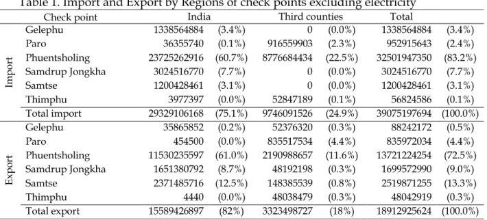
Bhutan’s trade heavily depends on India; most of its trade, constituting 83.2% of imports and 72.5% of exports, has gone via Phuentsholing, which is the nearest checkpost to enter India from Thimphu. This route has a long tradition, at least dating back to the 17th century.13 Table 1 shows the regionally aggregated
imports and exports at checkpoints. There are only two countries contiguous to Bhutan, which are India and China. Due to the territorial conflicts with China, official trade has ceased.14 The share of Indian trade constitutes 75.6% of imports and 82% of exports. Airport customs are located at Paro International Airport, and the amount of imports and exports appearing in Paro is totally by air freight. All the other imports and exports are by land transportation. Indian trade is
accomplished mostly by land. Trade with third countries via India is not subject to Indian custom duties.15 Trade with third countries by land transportation via India is not negligible: 22.6% of imports and 13.6% of exports.16
13 See Pommaret (1999) for more details on the trades before 20th century.
14 Pommaret (1999) and Sarkar and Ray (2012) mentioned the historical trade routes to Tibet from
Bengal plain.
15 It is allowed under the Agreement on Trade, Commerce and Transit between the Royal
Government of Bhutan and the Government of the Republic of India. See the original document at http://www.moea.gov.bt/documents/files/pub1xs9375dy.pdf.
16 We take the data for 2010 for the comparability of our following analysis benchmarked at 2010.
As of 2010, large fractions of exports as much as 75.8% are natural resources such as Ferro-silicon, calcium, Portland pozzolana cement, ingots, Portland slag cement, and others. On the other hand, imports are composed from small fraction of various commodities such as other light oils and Table 1. Import and Export by Regions of check points excluding electricity
Check point India Third counties Total
Im
p
o
rt
Gelephu 1338564884 (3.4%) 0 (0.0%) 1338564884 (3.4%) Paro 36355740 (0.1%) 916559903 (2.3%) 952915643 (2.4%) Phuentsholing 23725262916 (60.7%) 8776684434 (22.5%) 32501947350 (83.2%) Samdrup Jongkha 3024516770 (7.7%) 0 (0.0%) 3024516770 (7.7%) Samtse 1200428461 (3.1%) 0 (0.0%) 1200428461 (3.1%) Thimphu 3977397 (0.0%) 52847189 (0.1%) 56824586 (0.1%) Total import 29329106168 (75.1%) 9746091526 (24.9%) 39075197694 (100.0%)
E
x
p
o
rt
Gelephu 35865852 (0.2%) 52376320 (0.3%) 88242172 (0.5%) Paro 454500 (0.0%) 835517534 (4.4%) 835972034 (4.4%) Phuentsholing 11530235597 (61.0%) 2190988657 (11.6%) 13721224254 (72.5%) Samdrup Jongkha 1651380792 (8.7%) 48192198 (0.3%) 1699572990 (9.0%) Samtse 2371485716 (12.5%) 148385539 (0.8%) 2519871255 (13.3%) Thimphu 4440 (0.0%) 48038479 (0.3%) 48042919 (0.3%) Total export 15589426897 (82%) 3323498727 (18%) 18912925624 (100.0%) Notes: The values without parenthesis are in Nu and the values within parenthesis are the share in the total value.
3. Road projects
3.1. Road projects in Bhutan
There are several road projects within Bhutan, which appear in RSMP published by the Ministry of Works and Human Settlement (2006) and the Five Year Plan published by the Gross National Happiness Commission (2009, 2013, GNHC). There are five categories: 1) national highways, 2) dzongkhag roads, 3) farm roads, 4) thromde roads, and 5) access roads. 17 There are three subcategories within the first category: national highways. First is the international road connecting Phuentsholing to Thimphu, which is a part of Asian Highway numbered 48. Second is the primary national highway (i.e., East– West Highway and North–South Highway), and the third is secondary national highways (currently called district roads).
RSMP is a long-term plan, and detailed feasibility will be required to demonstrate its economic viability and determine exact specifications before individual projects can be implemented. With support from the Asian Development Bank (ADB), GNHC (2013) emphasized improvements to existing primary highways, secondary highways, and lower-categorized roadways.
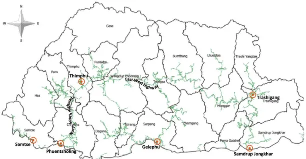
Figure 2: Current Road map of Bhutan
Source: by the authors based on maps from www.nsb.gov.bt
preparations (7.2%), ferrous products (3.2%), rice (2.2%), and others. See Table 2 of MFDRC (2010).
17 Thromde is a third level of administrative division in Bhutan followed by dsongdey (zone) and
Asian Highway No. 48, shown in figures 3 and 5, is the link between Thimpu and Phuentsholing and is called North–South Highway. It is also recognized as a part of the Bay of Bengal Initiative for Multi-Sectoral Technical and Economic Cooperation (BIMSTEC). Having its trade structure heavily dependent on the Phuentsholing border crossing, this highway is vital for the Bhutan economy. This is the top priority of the road improvements in Bhutan. Road construction started in the early 1960s in the first five-year plan as the first national highway. Since most parts of the road are single lane, construction of a bypass road is an on-going project. The bypass road between Chhukha and Damchu is yet to be completed.18 This road is connected beyond Thimphu. From Thimphu to the East, this section is called the East–West Highway, connecting to Trashigang in the East, which is also called the lateral road, National Road No. 1, and the Northern East–West Highway. After Thimphu, this road goes through Wangdue Phodrang, Trongsa, Bumthang, and Mongar between Thimpu and Trashigang.19
There is another important road called the Southern East–West Highway or the Second East–West Highway. Its planned length is 717 km; however, only 185 km has been completed, and another 194 km is under construction.20
3.2. Asian highway networks
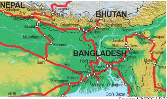
Asian highway networks (AHNs) can be seen as the compilation of prioritized national highways for international connectivity. Figure 3 presents the AHNs, published by UNESCAP in 2014. It depicts how the networks are connected among the regions. Further detailed maps of AHNs are shown in figures 4 to 6 for Bangladesh, Bhutan, and India.21
For Bhutan, the nearest international ports are Kolkata or Chittagong. Suppose there were only AHNs, the connectivity to Kolkata would require border crossing thrice and twice to Chittagong. However, of course, there are domestic roads from Bhutan–India border to Kolkata, and such roads are mainly used to avoid the redundant costs for further border crossings.
Since AHNs do not show regional connectivity within India, at least not in a practical sense, one must review the other road development plans and projects in India for such connectivity. In the following sections, we first review the subregional cooperation framework. Thereafter, the national project is briefly reviewed, with particular focus on Bhutan’s connectivity to Kolkata.
Figure 3: The Asian Highway Networks
18 A presentation at UNESCAP by a Bhutanese official, Wangdi and Wangchen (2013), is
available and informative. See Appendix II for some images of road conditions.
19 As is found in the following section, our simulation analysis is based on 2010 and simulated
till 2030. Some of the links are supposed to be built in the late 2020’s. See RSMP (2006).
20 See summary of transport sector in ADB (2013) for more details.
Source: UNESCAP 2014 Figure 4: The Asian Highway Networks in Bangladesh
Source: UNESCAP, AH Map of Bhutan
Figure 6: The Asian Highway Networks in India
Source: UNESCAP, AH Map of India
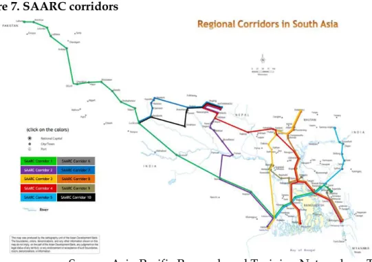
Ten roads are recognized by the SAARC corridors in South Asia (Figure 7). The following routes are listed from South (coast) to North (inland). SAARC Corridor 1 is from Agartala via Dhaka and Kolkata to Lahore. SAARC Corridor 2 is from Kolkata to Kathmandu. SAARC Corridor 3 is from Kolkata to Thimpu. SAARC Corridor 4 is from Chittagong and Mongla to Kathmandu. SAARC Corridor 5 is from Kolkata via Dhaka to Samdrup Jongkhar. SAARC Corridor 6 is from Chittagong to Agartala. SAARC Corridor 7 is from Lucknow via Nepalgunj to Kathmandu. SAARC Corridor 8 is from Chittagong and Mongla to Thimpu. SAARC Corridor 9 is from Maldah to Sirajganj. SAARC Corridor 10 is from Lucknow via Gorakhpur to Kathmandu.
Figure 7. SAARC corridors
Source: Asia-Pacific Research and Training Network on Trade http:/artnet.unescap.org/tid/projects/transit-collab-cuong.pdf
From this list, corridors 3 and 8 are the projects within the region focused on in this paper. When we evaluate the impacts on landlocked Bhutan, SAARC Corridor 3 strengthens the connectivity between the Kolkata port in India and Bhutan. SAARC Corridor 8 also serves to Bhutan for the shipments via the Chittagong port in Bangladesh; however, the competitiveness of SAARC Corridor 8 against Corridor 3 is relatively lower. First, the distance of Corridor 8 is longer by approximately 100 km, and some parts of road conditions are inferior in Bangladesh than those in India. Second, the number of border crossings is increased by one, and this border crossing is not as easy as transportation within India.
improve the accessibility of northeastern India to all the international markets. On the other hand, Corridor 8 mainly improves accessibility to Bangladesh and also serves to the southern part of northeastern India to connect international market via the Chittagong port. The presence of an international border is a challenge that magnifies the clear improvement. We have also included the scenario for Corridor 8 to examine the overall impacts of SAARC corridors in this region.
3.4. West Bengal Corridor
Figure 8: West Bengal Corridor
Source: Asian Development Bank (2012)
costs,” “improving road safety,” and “reducing travel time.”22 These benefits are typical direct effects of roadway improvements. Figure 8 depicts a map of West Bengal Corridor.
Given that more than 70% of imports and exports pass through India, a large percentage of such transportation may use this West Bengal Corridor from the Kolkata port to Phuentsholing. The improvements at this intersection would impact freights to Bhutan.
4. The model
We have employed the model of NEG, which captures the agglomeration economies of firms and people. This feature is indispensable for the regional analysis of Asia because we have observed that the dynamic developments in Asia can be characterized by urbanization and industrial agglomeration (clustering). Our model is naturally multiregional and multisectoral23.
The theoretical foundation follows the study by Puga (1999), which captures multisector and country general equilibrium of NEG with costly agricultural goods. Instead of including transportation of agricultural goods as a variable (Puga, 1999), we have introduced land size as an input for agriculture. The idea behind and hypothesis of these types of models is that total concentration of all activities shown by the typical NEG models may be unrealistic.24 Since this paper applies this model for the case of developing regions in Asia, the model is formulated as such. Agricultural land rent is assumed to belong to the households in the same region.
There are seven sectors within the model: agriculture, five manufacturing sectors, and the service sector. It allows for worker mobility within countries and between sectors but not among countries.
Although transport of agricultural goods is assumed to be costless, the transport of manufactured goods and services is assumed to be of the iceberg type. All products in the three sectors are tradable. On the one hand, transport costs for agricultural goods are assumed to be zero and the price of agricultural goods is chosen as the numeraire, implying that the price of a good is the same in each regional economy. On the other hand, transport costs of manufactured goods and services are assumed to be of the iceberg type. That is, if one unit of product is transported from one location to another, only a portion of the unit arrives. Transport costs within the same region are considered to be negligible.
In this setup, regional incomes of location r can be expressed as follows:
!(#) = &'(#)('(#) + *+(#),+(#) + *-(#),-(#) (1)
where &'(#) denotes the price of an agricultural product derived from location
22 Asian Development Bank (2012:1).
23 For other simulation analysis based on NEG, see for example Teixeira (2006) and Robarts et al
(2012).
r at location r, ('(#) represents agricultural products at location r, *+(#) and
*-(#) are nominal wage rates in the manufacturing sector and the services sector
at location r, and ,+(#) and ,-(#) are labor inputs in the manufacturing sector and the services sector at location r, respectively25. In our simulation, regional income corresponds to regional GDPs.
The price indices of agricultural goods, manufactured goods, and service goods at location r are expressed as follows:26
.'(#) = /∑ 16785 '(#)2345&'(#)4(2345)97:'4(2345);
<
=(>3=<), (2)
.+(#) = @A ,+(B)1+(#)2C45*+(B)(542C)D.+(B)42C(54D)9:7+4(2C45)
6
785
E 5
4(2C45)
and, (3)
.-(#) = /∑ ,6785 -(B)1-(#)2J45*-(B)4(2J45)9:7- 4(2J45);
<
=(>J=<), (4)
where &'(#) = /K'∑6785!(B).'(B)234597:'4(2345)/('(#); <
(>3=<), M denotes the
input share of labor in producing manufacturing goods; K' denotes the consumption share of agricultural products; 1', 1+, and 1- are productivity parameters for location r; 97:', 9:7+, and 9:7- denote the iceberg transportation costs from location r to location s; and N', N+, and N- are the elasticity of substitution between any two differentiated manufactured goods for agricultural goods, manufactured goods, and service goods, respectively. Nominal wages in the agricultural, manufacturing, and services sectors at location r are expressed as follows:
The aforementioned variables have been calculated with actual or estimated data and parameters and, in the model, the workers choose their best location and the sector to work. The dynamics of labor to decide on a specific sector within a location is expressed as follows:
*'(#) = O1'(#) PRQ(:)
3(:)S
54T
&'(#), (5)
*+(#) = U'C(:)D
<
>C/∑[Y\<V(7)WXYC<=>CZC(7)=(<=>C); < >C
ZC(:)<=] ^
< ]
, and (6)
*-(#) = 1-(#)/∑ !(#)96785 :7- 542J.-(B)4(542J);
<
>J. (7)
where `ȧ (#) denotes the change in labor (population) share for a given sector
25 Except the introduction of agricultural land rents, this regional income equation is typical
among the similar models.
within a location, ca denotes the parameter used to determine the speed of switching jobs within a location, da(#) denotes the real wage rate of any sector at location r, de(#) denotes the average real wage rate at location r, and `a(#) denotes the labor share for a sector in the location. The population share for a sector within a country is expressed as follows: `a(#) = R Rf(:)
3(:)gRC(:)gRJ(:), where
,'(#) denotes labor input of the agricultural sector at location r. Then, the
dynamics of labor migration between regions is expressed as follows:
`ȧ (#) = caPhhe(:)f(:)− 1S `a(#), k ∈ {1, n, o}, (8)
where `Ṙ (#) denotes the change in the labor (population) share of a location in a country, cR denotes the parameter for determining the speed of migration between locations, and `R(#) denotes the population share of a location in a country. The symbol deq indicates the average real wage rate at location r, and
d(#) indicates the real wage rate of a location and is specified as follows:
d(#) = r(:)/sR3(:)gRC(:)gRJ(:)t
Z3(:)u3ZC(:)uCZJ(:)uJ (10)
where K+ and K- indicate the consumption share of manufacturing and services, respectively.
5. Data, parameters, simulation procedure, and scenarios
5.1. Data
For our simulation, the most crucial variables are population, regional gross domestic product (RGDP), its industrial composition, and the size of arable lands. The main focus of our analysis is the 18 countries or regions in East, Southeast, and South Asia. For these areas, we have regional data. More specifically, the administrative units adopted in the simulation are one level below the national level for Cambodia, Japan, Korea, Lao PDR, Malaysia, the Philippines, Taiwan, Thailand, and Vietnam. For Bangladesh, China, India, Indonesia, and Myanmar, the administrative units are two levels below the national level. Brunei Darussalam, Hong Kong, Macau, and Singapore are treated as one unit.
Source: Authors’ calculation
At these administrative levels, we have constructed industrial composition data for seven sectors: agriculture, five manufacturing sectors, and services. Five manufacturing sectors are automobile, electrical & electronic equipment, textile, food processing, and other manufacturing. The data are constructed either from original public statistics or the elaboration with available public data. When data by region and by industry is not available, we can obtain any supplementary survey to decompose RGDP, such as manufacturing surveys or an economic census.27 Our data also includes more than 60 countries other than those in East Asia. These countries are treated as one region by each.28 Furthermore, there are approximately 1,800 regions in our dataset. Our baseline data is for 2005 and we have run simulations until 2010 to calibrate the actual national GDP in 2010.
5.2. Data for Bhutan
We have compiled Bhutan data for this paper. This is because sector-wise
27 In principle, we have obtained regional industrial quotient by supplementary data, which may
be aggregated from microdata. Then, we have divided RGDP by this quotient. Details in the construction of data and sources are explained by each country. See the following website;
http://www.ide.go.jp/English/Data/Geda/make.html. The data used in this simulation is aggregated into seven sectors.
and region-wise governmental data is not fully available. The district centers are defined as the point expressing the highest population density in the district. The distances are obtained using the road data among the district centers. The population data utilize LandScan 2010.
For the construction of industrial decomposition and regional distribution of each industry, we have faced difficulties due to the lack of data availability. Yet, we have used remote sensing technique to construct such data. For agricultural production among the districts, we have utilized land coverage data of cropland and related categories from a MODIS’s land cover dataset (MCD12Q2) in 2010. We have considered the land coverage of vegetation as a proxy for the regional distribution of agricultural activities and have aggregated it for each administrative unit. Taking the regional share of the land size for vegetation as the multiplier, the GDP of agriculture has been distributed among the regions. For the regional distribution of manufacturing activities that may intensively use electricity, we have employed the nighttime light as a proxy. This has been obtained from Defense Meteorological Satellite Program-Operational Linescan System, which was processed and published by the National Geophysical Data Center in 2010. We have aggregated the nighttime light intensity for each administrative unit and have made the regional share of nighttime light intensity. Taking this regional share as the multiplier of manufacturing activities, we have distributed the industrial value added at national level over districts. The composition of the GDP by industry at the regional level was assumed to be the same as the sectorial share of Bhutan’s exports at the national level (at the initial baseline year), which was computed from HS six-digit export data obtained from COMTRADE in 2010.29 The shares were set as follows: automobile (0.48%), electrical and electronic equipment (0.44%), textile (0.33%), food processing (2.48%), and other manufacturing (96.28%). In the service sector, the same methodology with nighttime light was deployed to find the geographical distribution of economic activities. Similarly, using this multiplier, the GDP of the service sector was distributed across districts. Finally, district-specific GDP by sector was complied.
Figure 10. Estimates of Real GDP at 2010 for Bhutan and her surroundings
29 Unfortunately, we could not find any information about regional distribution of
Source: Authors’ calculation
5.3. Parameters
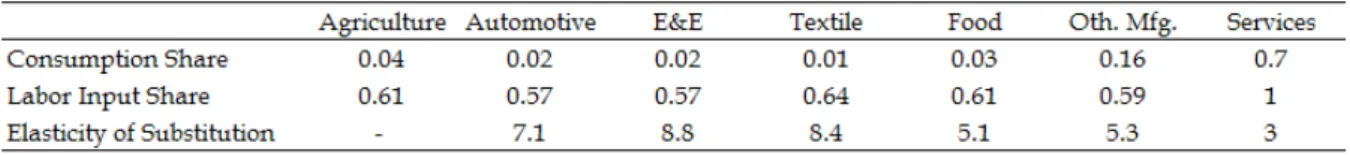
There are mainly three types of parameters in our model; consumption, production, and modal choice. Specifically, these parameters represent the expenditure share for the different commodities, labor-capital ratio of industries, elasticity of substitutions for goods, and cost parameters of transportation over its different modes.
The consumption shares of consumers over different commodities are uniformly determined for the entire region in the model. It would be more realistic to change the share by country or region; however, we cannot do so because we lack sufficiently reliable consumption data at finer levels of geographical units. Similarly, labor input share for each industry is uniformly applied throughout the entire region and a single time period in the model.30 Although it may differ among countries or regions and across time, we have used an “average” value: in this case, the value for Thailand, which is a country in the mid-stage of economic development and whose values are taken from the Asian International Input–Output Table for 2005 by the IDE-JETRO. For the manufacturing sector data source, we have used the survey conducted by the JETRO (2013).31 We have mainly adopted the elasticity of substitution for the
30 The changes in these parameters may affect the speed and degree of agglomeration because
they are the determinants of centrifugal forces. See the equation called “break point” of the models in Fujita et al (1999) and Behrens and Robert-Nicoud (2001). With our theoretical setting, larger expenditure share and smaller labor input ratio for increasing returns to scale sectors would strengthen the centrifugal forces.
31 The difference between the benchmark and the real parameters in these parameters may work
manufacturing sectors from the study by Hummels (1999) and have estimated it for services.32
Table 2. List of parameters for consumption and industry
Source: authors’ calculation
Our transport costs comprise the physical transport costs, time costs, tariff rates, and non-tariff barriers. Physical transport costs are a function of distance traveled, travel speed per hour, physical travel cost per kilometer, and holding costs for domestic/international transshipments at border crossings, stations, ports, or airports. Time costs depend on travel distance, travel speed per hour, time cost per hour, and holding times for domestic/international transshipments at border crossings, stations, ports, or airports. These parameters were derived from the ASEAN Logistics Network Map 2008 by the JETRO and by estimating the model of the firm-level transport mode choice using the “Establishment Survey on Innovation and Production Network” (ERIA) for 2008 and 2009, which includes manufacturers in Indonesia, Philippines, Thailand, and Vietnam.33
5.4. Simulation procedure
The simulation involved a repeated two-step procedure. During the first step, with given distributions of employment and RGDP by sector and region, a short-run equilibrium was obtained. For the second step, observing the achieved equilibrium, workers migrate to regions and industries according to differences in real wages. This migration of people brings us the updated distribution of employment and RGDP. In our simulation model, these two steps correspond to one year. We have repeated this procedure until 2030 with some fundamental assumptions that are mentioned in the next section.
5.5. Baseline scenario and fundamental assumptions
of concentrations in people and firms. However, such changes may be marginal as long as the difference is negligible. At least, we have executed several sensitivity analyses and as long as the changes in parameters are marginal, the differences in the results are negligible.
32 Estimates for the elasticity of services are obtained from the estimation of the usual gravity
equations for trade services, including independent variables such as the importer’s GDP, the exporter’s GDP, the importer’s corporate tax, and the geographical distance.
33 See Table 2 in the study by Kumagai et al (2013) for specific parameters and Kumagai and
We have some of the fundamental assumptions for our simulations in every scenario. 1) National population of each country is assumed to increase at the rate forecasted by the UN Population Division until the year 2030. 2) International migration is prohibited.34 3) Tariffs, non-tariff barriers, and services barriers change based on the FTA/EPAs currently in effect. 4) Exogenous growth rates on technological parameters are specified by each country to calibrate the GDP growth trend from 2005 to 2010.
5.6. Scenarios for road improvements within Bhutan
The five-year plan of Bhutan indicates several development issues. Most of the roads are still restricted to one lane. This creates obstacles to other vehicles and reduces the average speed. The improvements may include the expansion of lanes, shortcuts that reduce overall distance, and the construction of tunnels. We have assumed that all such investments contribute to the increase in speeds from low level (19.5km/h) to intermediate level (38.5km/h) when all the necessary construction is completed.35 This intermediate level of average speed is the one obtained on standard roads in Thailand. Scenario 1 is the link between Phuentsholing and Thimphu. This is the best conditioned road in Bhutan. From the available information, we have set the average speed of this route in 2010 at 25 km/h.36
Scenario 1: Bypass construction of North–South Highway, Thimphu and Phuentsholing
Scenario 2: Upgradation of National Road No.1, Thimphu–Trashigang Scenario 3: Second East–West Highway, Samtse–Samdrup Jongkhar37
Scenario 1 is exactly included in the project supported by the ADB under BIMSTEC. For more intuitive images, typical road conditions of some main roads are shown in Appendix II. This includes the bypass construction between Damphu and Chhukha, and its completion shortens the road distance from 179
34 The migration parameter is taken from the study by Barro and Sala-i-Martin (1992) and
calibrated to copy the actual population growth in representative cities during 2005-2010. Barro and Sala-i-Martin1992estimated the inter-state migration rate in the US responding to a 10% difference in the income as 0.26 and the inter-prefecture migration rate in Japan as 0.27. We have calibrated the number to 0.20.
35 Actual drive from Thimpu to Damchu in June 2015 was 40 km/h.
36 From a movie in YouTube, https://www.youtube.com/watch?v=rTnJdWSOba8, posted on
January 2015, we can understand that passenger buses operated to Thimphu from Phuentsholing, which is 170km, by 6 hours’ drive. This means that average speed was about 30 km/h. Since there is an ongoing improvement of roads, the average speed may be continuously increasing. Having these presumptions, we have set the average speed as 25 km/h in 2010.
37 We have drawn the highway from Samtse, Phuentsholing, Chhukha, Dagana_Junc, Sarpang,
km to 159 km.38
Scenarios 2 and 3 are prioritized projects listed in the Road Sector Master Plan 2007–2027, which is published by the Ministry of Works & Human Settlement, Royal Government of Bhutan in 2006.
Scenario 4: Trade facilitation at border crossing posts (i.e., Phuentsholing, Gelephu, and Samdrup Jongkhar)
Scenario 4 deals with the improvements in the non-physical institution. In our analysis, most developing countries in Southeast Asia have achieved a clearance time of 13 hours at the border post, on average. After modernization, harmonization of process, and other improvements, border post may reduce the clearance time by one-half (6.5 hours). From the interviews and observations, crossing the Bhutan border may require additional hours. We have assumed that the clearance time at the Bhutanese border is 26 hours. After the facilitation efforts, we have assumed that the level of effectiveness is just as good there as it is at the other border posts in Asia, where the clearance time has become 6.5 hours. Moreover, the loading costs reflecting the change of the containers are specified as twice of the average cost in ASEAN countries.39 More precisely, on the one hand, loading costs in other countries are assumed to be 500 USD per container and can be 250 USD per container with improvement in investments. On the other hand, Bhutan is assumed to have a loading cost of 1,000 USD per container and can be improved to 250 USD per container.
Scenario 5: Construction of SEZ at Pasakha in Chhukha
Similar to other developing countries in Asia, there is a project to construct special economic zones (SEZs) at Pasakha in Chhukha. Scenario 4 assumes the construction of such an industrial zone in Pasakha to set the regional productivity in Chhukha at 1.2 times. The assumption of such exogenous growth in regional productivity means an annual increase of 0.11% in labor productivity, which may result in encouraging domestic investment, foreign direct investments, technical assistance for training, and other benefits. The impacts on regional economies from SEZ have supporting evidence (Wang, 2013).40
5.7. Scenarios for road improvements in India
Scenario 6: Upgradation of SAARC Corridor 3 to Kolkata
38 This section is 15% of the link between Thimphu and Phuentsholing. Supporting information
on the length of this road can be found in the study by Wangdi and Wangchen (2013).
39 Loading Costs is set as the time and money costs of transshipment, which is estimated by our
team from JETRO (2008) of the ASEAN Logistics Network Map.
SAARC corridors may well be implemented as planned. The national transport development policy committee in India (2014) emphasized the connectivity within Southeast Asia and the improvements of logistics networks within its North East regions. This planning was determined within the context of Indian national politics. Note that for this scenario, the trade facilitations with Bhutan and India are not assumed to be implemented.41 Thus, Scenario 5 considers the spillover effects of the Indian infrastructure project on Bhutan. Current assumption regarding the average speed on main Indian roads is 38.5 km/h. The improvements would likely facilitate a speed of 60 km/h.42
5.8. Scenarios for combinations of some measures
Scenario 7: All of road developments in Bhutan (scenarios 1 to 3)
Scenario 8: Road developments and trade facilitations (scenarios 1 to 4) Scenario 9: Trade facilitations and SAARC Corridor 3 (scenarios 4 and 6) Scenario 10: Road developments and SAARC Corridor 3 (scenarios 6 and 7) Scenario 11: Road developments, trade facilitations, and SAARC Corridor 3 (scenarios 4, 6, and 7)
As the Road Sector Master Plan was drawn, several development projects were being implemented at the same time. Note that the scenarios listed in previous sections examined individual impacts. We have examined the combination of some measures. Scenario 7 can be understood as the combined impacts of major roads in the Road Sector Master Plan. Scenario 8 is the combination of road development and trade facilitations. These two are the domestic efforts to ameliorate accessibility of products from Bhutan to foreign markets.
How can we expand the benefits provided by outsiders? While Scenario 9 combines SAARC Corridor 3 with trade facilitation, Scenario 10 combines with road developments. Finally, Scenario 11 combines all road developments linked to SAARC Corridor 3.
Scenarios 9 to 11 consider the combined results with SAARC Corridor 3. Scenario 11 considers the spillovers of SAARC Corridor 3 with better border environments by trade facilitations. This enables us to examine how Indian development contributes to the increase in the accessibility of Bhutan and how it can be magnified by lowering transaction costs at Bhutan’s border. Scenario 10 considers the combined results with road developments instead of trade facilitation. Scenario 11 considers road developments and trade facilitations with
41 As a country ranked as 126 in 2010 and 125 in 2015 by Doing Business, it is easily inferred that
transaction costs to cross the border are very high. This is a critical factor preventing the positive spillover from India. Any investments in the facilitations at the border crossing would reduce the costs and allow to inflow the benefits. See more on scenario 11 for the combination with trade facilitation in scenario 4. See also Wilson et al (2003).
42 This average speed is based on the sample survey of actual driving at similar level of roads
SAARC Corridor 3. Road development and trade facilitations may have shown some progress at the same time, the most plausible scenario.
6. Results
Our simulation results for each scenario reveal the geographical extent of increased accessibility measures, directions of migration, and the economic impacts. Since the accessibility measure for each district is defined by the sum of each market size discounted by the distance for all of the other districts, the accessibility measure of each district changes when there are any logistical improvements in any part of the network. However, the magnitude of improvement in the accessibility measure should differ depending on the proximity to the improved link and the size of the market that will, in effect, become closer due to improvements. The changes in accessibility affect the profitability of firms, labor demand, and labor wage rates. Hence, people and firms relocate to their best location. This means that the direction of migration can be changed with logistical improvements.43 This change in direction of migration may be called a diversion effect—a notion similar to that in international trade when custom unions or FTAs cause changes in trade patterns.
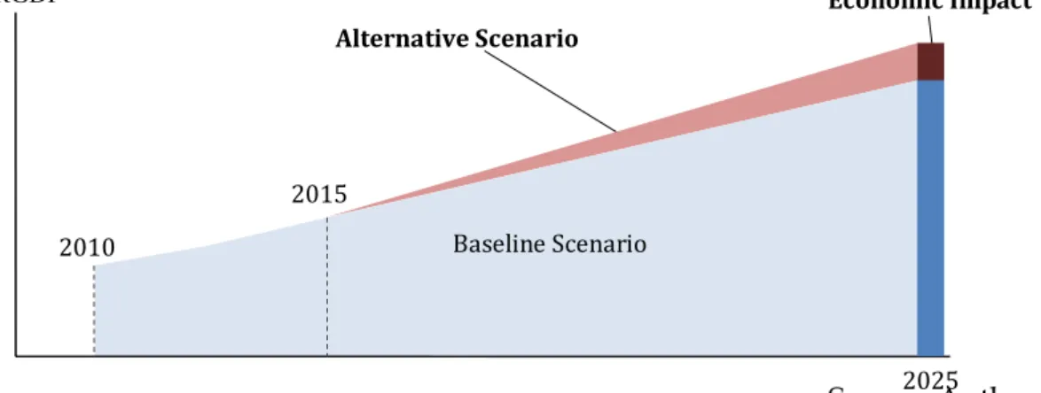
We have performed simulations to estimate the RGDPs by industry for each scenario and show the differences with the baseline scenario. The baseline is taken as the without-project scenario and is assumed to be the minimal additional infrastructure development accomplished after 2010. The alternative scenarios contain specific policy measures in 2015 and beyond. We have compared the RGDPs between two scenarios in 2030. If the RGDP of a region under one scenario is higher (lower) than that under the baseline scenario, we regard the surplus (deficit) as positive (negative) economic impacts of the project (Figure 11). If a region has a negative economic impact from a project, it does not mean that the region is worse off compared with the current situation but rather indicates relatively slower growth compared with the baseline scenario. As is seen in Section 2, Bhutan has achieved high economic growth and will most likely achieve similar economic growth. Negative values in the results simply imply relatively slower growth compared with the baseline scenario.
43 To make the following discussion clear, a brief example is shown here. Under the baseline
Figure 11: Image Diagram: Difference between the Baseline and Alternative Scenarios (a case for positive impacts)
Source: Authors.
We have listed two sets of scenarios. One deals with physical infrastructure improvements and the other with non-physical improvements. First, physical infrastructure improvements are mainly restricted to road improvements in this region, including better bridges. So, it is all about upgrading roads and building new ones. On the one hand, it can be separated into two parts by its territorial implementation. One is within Bhutan, and the other is in either Bangladesh or India. The project within Bhutan affects internal economic geography. On the other hand, the external project of Bhutan can also affect it. Second, non-physical improvements comprise forms of institutional reforms, including harmonization of trade processes, electrification and digitalization of customs processes, and so on. Such reforms can reduce the non-tariff barriers and may enhance trade and accessibility.
In the context of Bhutan’s governmental policy, this analysis employs the measure for the analysis only in monetary terms. It inherently encloses the limitation of the choice of the variables to evaluate people’s happiness. It is highly desirable to link the model with other socioeconomic variables such as health conditions, education attainments, consumption behaviors, and income levels. However, the lack of empirical and theoretical links with economic variables has limited the analysis.
In the following sections, all the maps indicate the comparisons of real RGDP per capita under each scenario with respect to the estimated baseline in 2030, which is the ratio of RGDP to the without-project scenario. The simulated numbers in the maps are attached in Appendix III (tables).
6.1. Scenario 1: Road improvements between Thimphu and Phuentsholing
Scenario 1 improves the connectivity from Thimphu to Phuentsoling by building the bypass between Damchu and Chhukha. Overall, improvements enable reductions in distance traveled and travel costs and time to and from India. As discussed in Section 2, Thimphu and Phuentsholing are the two polar cities in
2010
2015
Baseline Scenario
Alternative Scenario
2025
Bhutan, and this scenario strengthens the connectivity between them. The results show that increased connectivity between the two cities enables national economies to expand and make imported goods more reasonably priced. This effect is observed by the positive effects found in most regions. The results indicate that population growth is higher in Chhukha and Samtse. Due to increased accessibility, there may be more migrants heading toward Chhukha and Samtse. Indeed, the total number of migrants has increased. While some of them were supposed to go to Thimphu or other neighboring regions, the changes in expectations may bring people toward Chhukha and the surrounding regions, i.e., diversion effects.
Since the corridor from Thimphu to Phuentsholing increases relative accessibility, these regions grew more than that under the baseline. The magnitude of growth in Chhukha was largest and that in Thimphu was second. This is because of the negative impact of the diversion effects on Thimphu by reducing migration and positive impact on Chkkuhka by increasing in-migration. Relative improvements in the West are associated with the opposite outcomes in the East. Associated changes compared with those in the baseline (without the project) is shown to be negative only in one region in the East: Pemagatshel.
Figure 12. Economic impact of Scenario 1
Source: Authors’ calculation.
6.2. Scenario 2: Upgradation of National Road No.1
accessibility to larger markets are higher in the East. There are other clear impacts in both the North and the South. Since these regions are not directly improved by the project, relative accessibility is decreased. Thus, there are negative effects. This project can have an offsetting effect within Bhutan under Scenario 1 by making eastern parts more viable, resulting in more people migrating to the eastern parts compared with the baseline scenario. Note that only Samdrup Jongkhar and Gasa may decrease its real RGDP per capita compared with the baseline but the real RGDP per capita of Samtse and Sarpang may be unchanged.44
Figure 13. Economic impact of Scenario 2
Source: Authors’ calculation.
6.3. Scenario 3: Second East–West Highway
The construction of the Second East–West Highway would increase accessibility among the southern districts. Without such highway, these regions would not be able to connect directly within Bhutan and one would have to use Indian roads. We can observe that there are significant impacts. Pemagatshel
44 There may be some out-migration from these regions but the out-migration contributes to keep
does not connect directly via the Second East–West Highway and has negative impacts, which may suggest out-migration to border regions.
Contrary to Scenario 2, Samdrup Jongkhar would enjoy an increase in accessibility, in-migration, and growth in real RGDP per capita. Ha, Thimphu, Trashi Yangtse, and Trongsa might experience some out-migration but will still retain the same level of real RGDP per capita. The simulation results also indicate that there may be diversion with regard to border crossings from Phuentsholing to Samdrup Jongkhar. If such diversion in trade flows happen, the impacts may be in line with this result. However, if the logistical structures persist in their current form, the shift to Samdrup Jongkhar may not be sufficient to sustain this result, leading to middle or lower results.
This scenario can be a good complement to the previous scenarios because the most positively affected regions are the ones that cannot go lower under the two scenarios.
Figure 14. Economic impact of Scenario 3
Source: Authors’ calculation.
6.4. Scenario 4: Trade facilitation at border posts (Phuentsholing, Gelephu, Samdrup Jongkhar)
that regions are linked to each other in space.
Due to cheaper availability of imported goods, most regions enjoy an increase in real RGDP per capita.
Similarly, under Scenario 3, Samdrup Jongkhar increases its position as a border crossing. Sarpang also increases its position as the host of Gelephu border crossing. The key to this is the flexibility of the transportation sector and the supply chain related to imported commodities.
Figure 15. Economic impact of Scenario 4
Source: Authors’ calculation.
6.5. Scenario 5: Construction of SEZ at Pasakha in Chhukha
Scenario 5 considers an increase in regional productivity at 20% in Chhukha, which reflects the possible construction of SEZ at Pasakha. The SEZ at Pasakha is assumed to be as productive as the ones in Chinese examples in the study by Wang (2013).45
SEZ has significant positive impacts in Chhukha, and all other regions are as good as in the baseline case. While there is out-migration from the rest of Chhukha, the real RGDP per capita of the other regions remains the same. The
45 It should be mentioned that it is not only SEZ but the linkage with the local economies may
diffusion of positive effects is insignificant. It may depend on production networks, i.e., the demand from SEZ increases the production of surrounding regions. The results capture both labor demand and in-migration to Chhukha. Since the model assumes the intra and interindustrial linkage for their production, such industrial linkage can magnify the impacts. This industrial linkage totally depends on the local structure of industries.
Figure 16. Economic impact of Scenario 5
Source: Authors’ calculation.
6.6. Scenario 6: Upgradation of SAARC Corridor 3 from Bhutan border to Kolkata
Bhutan.46
This result in Bhutan provides an interesting example that can be considered while implementing policies for landlocked countries. The infrastructure improvements in transit (gate) countries favoring landlocked countries have a much stronger impact on the frontier regions in the transit countries. In the case of North East India, the government has the long-term infrastructure plan, which insures better accessibility to Bhutan.
Figure 17. Economic impact of Scenario 6
Source: Authors’ calculation. 6.7. Scenario 7: All road developments in Bhutan (scenarios 1 to 3)
Scenario 7 sums up three domestic road development scenarios. There is only one region in the North, Gasa, which shows a negative outcome. It is isolated from the road network (Figure 2) and cannot benefit from the projects. All the other regions can benefit from them.
Notably, the previous results have indicated that the impacts differ from the implementation of scenarios 1 to 3. In their individual results, there are
46 To consider the possible reaction of Bhutan to garner the positive impacts from SAARC
disparities in impacts from positive to negative. However, since all of these scenarios can work complementarily, most regions can benefit from the projects: Scenario 1 contributes to the western parts, Scenario 2 contributes to the eastern parts, and Scenario 3 contributes to the southern parts. This brings more regional development and reduces the polarization of Bhutan.
Since we have not included feeder road projects, which are listed in the Road Sector Master Plan, the actual impacts may be larger than those under this scenario. When we include feeder roads, even Gasa would be further connected to other regions.
In sum, the current RSMP projects can better connect the regions and can allow regions to enjoy economic growth and facilitate people to migrate for better opportunities.
Figure 18. Economic impact of Scenario 7
Source: Authors’ calculation.
6.8. Scenario 8: Road developments and trade facilitations (scenarios 1 to 4)
The following regions saw positive increases with the additional policy measures of trade facilitation: Trashigang, Zhemgang, Pemagatshel, Dagana, Paro, Trongsa, Tsirang, Wangdue Phodrang, Chhukha, Sarpang, Thimphu, and Samdrup Jongkhar. The largest regional impacts were on Samdrup Jongkhar and Thimphu.
Moreover, there were no effects on Indian regions, implying that Bhutan may not be an important market for India’s surrounding regions as much as India is for Bhutan.47
Figure 19. Economic impact of Scenario 8
Source: Authors’ calculation.
6.9. Scenario 9: Trade facilitations and SAARC Corridor 3 (scenarios 4 and 6)
This scenario was performed to compare the results with and without trade facilitation. Trade facilitation would allow Bhutan to have more diffusional impacts from the road construction of SAARC Corridor 3. The positive impacts would mainly prevail in internal districts. This is one of the possible outcomes of the ongoing projects. In this scenario, even without implementing road development projects within Bhutan, trade facilitation would become key to
47 This may be contrary to the ancient time trades, where trade connection to Cooch Behar and
garner the positive impacts from India and spread them to internal districts. All the regions except Gasa can benefit from these improvements. The synergy effects emerge at Chhukha, where the impacts are larger than the sum of both improvements.
Figure 20. Economic impact of Scenario 9
Source: Authors’ calculation. 6.10. Scenario 10: Road developments and SAARC Corridor 3 (scenarios 1 to
3 and 6)
The direction of regional impacts is similar to that in Scenario 9, but the magnitudes are larger in this scenario. Almost all the regions have experienced positive effects. The impacts are even larger than those in Scenario 9 once the SAARC Corridor 3 completion is combined with trade facilitations. This difference in the combination with trade facilitations or road developments captures the mountainous terrain within Bhutan, which prevents internal connectivity. With additional infrastructure improvements within Bhutan, the impacts are far larger than the ones in North East India.
The synergy effects are found at Gasa, Trashigang, Lhuentse, Punakha, Wangdue Phodrang, Sarpang, Bumthang, Mongar, Trashi, Yangtse, Thimphu, Chhukha, Samdrup Jongkhar, and Samtse. Other regions such as Dagana, Ha, Paro, Pemagatshel, Trongsa, Tsirang, and Zhemgang show slightly lower impacts than the sum of each. This result can again be a good example of successful cooperative and strategic partnership with a landlocked country and a transit country, which can magnify the impacts in the landlocked country from both physical and non-physical infrastructure improvements within both countries.
Figure 21. Economic impact of Scenario 10
Source: Authors’ calculation. 6.11. Scenario 11: Road developments, trade facilitations, and SAARC
Corridor 3 (scenarios 1 to 5 and 6)
Figure 22. Economic impact of scenario 11
Source: Authors’ calculation.
7. Policy implications of the analysis
Unlocking landlocked countries and regions is a challenge for geographically disadvantaged people. This study provides an evaluation of ongoing road infrastructure projects, institutional reforms, and possible positive productivity shocks in Bhutan.
Better accessibility insures easier access not only to basic materials but also to more imported goods. Road infrastructure improvements within Bhutan are found to be very important, bringing greater impacts compared with those under trade facilitations. This fact occurs because the changes in accessibility are bigger.
the Southeast–West Highway, serves to differentiate the regions and enhance regional connectivity, bringing benefits to entire districts. Consequently, any expected induced migration can be reduced.
Scenario 4 has confirmed that easier trade at border posts can bring benefits from trade throughout the regions in Bhutan. Scenario 5 shows the possible regional impacts of SEZ, which are positive and locally significant. Scenario 6 shows that road projects in India can improve the accessibility of Bhutanese regions to imported and exported goods and can bring positive impacts to them. Compared with the regions in North East India, the regions in Bhutan benefit less. This may be explained by the mountainous terrain and high non-tariff barriers between Bhutan and India.
We have also examined some combinations of projects. It is confirmed from the results that Bhutan can benefit from Indian road projects and can magnify the impacts if road developments, trade facilitation, or both may be implemented. Particularly, the road developments have significant impacts compared with trade facilitations.
From the results of all scenarios, the combinations of the several development projects can comprehensively increase the accessibility to and economic growth in the regions. Although there are international borders in the regions, the effects of the infrastructure improvements can be transmitted across the borders. How far such a diffusion effect can be transmitted depends on domestic road networks, non-tariff barriers at the borders, and internal transportation conditions.