野外データにもとづく森林動態のモデリング

九州大学学術情報リポジトリ

Kyushu University Institutional Repository

野外データにもとづく森林動態のモデリング

久保, 拓弥

九州大学理学研究科生物学専攻

https://doi.org/10.11501/3134901

出版情報：Kyushu University, 1997, 博士（理学）, 課程博士 バージョン：

権利関係：

Forest Dynamics Models Based On Field Measurements

TAKUYAKUBO

Department of Biology Faculty of Science Kyushu University Fukuoka 812-81, Japan

Dissertation

submitted in partial fulfillment of the requirements for the degree of

DOCfOR OF SCIENCE in Biology

Division of Science,

Graduate School of Kyushu University

Contents

I. Preface . . . .. . . ... . . ... . . ... . . .. . ....... . . 1

II. Forest Spatial Dynamics with Gap Expansion: Total Gap Area and Gap Size Distribution 2.1. Introduction ...^....^{. .}..^....... . . .... . . ...... . . ..^{. .}..^{. . .}..^..^{. . . .}...^...^....^{. .}... 6

2 .2. Model ..^{. . . . .}.^{. . . .}..^{. . .}.^......^..^..^{. .}.. . . ... . . ....^{. . . . .}.^{. .}.^..^..^{. . .}.... ......^...^{. . . .}..^. 9

2.3. Total gap area ... 12 2.4. Cornputer simulation . . . . 16

2.5. Supply-dependent recruitment and bistability . . . . 18

2.6. Gap size distribution . . . 20

2. 7. Discussion .. . . . ...^..^...^..... . . .........^{. .}..^..^{. . .}.^...^...^{. .}...^...^{. . . . .}..^....^......^{. .}. 24

Appendix A: Proof of the inequalities for local and global densities . . . . 31

Appendix B: Analytical solutions from pair approximation ( 1) ...^..^...^...^...^..^..... 32

Appendix C: Analytical solutions from pair approximation ( ²) ... 34

Appendix D: Maximum likelihood estimation of site transition rate . . . 36

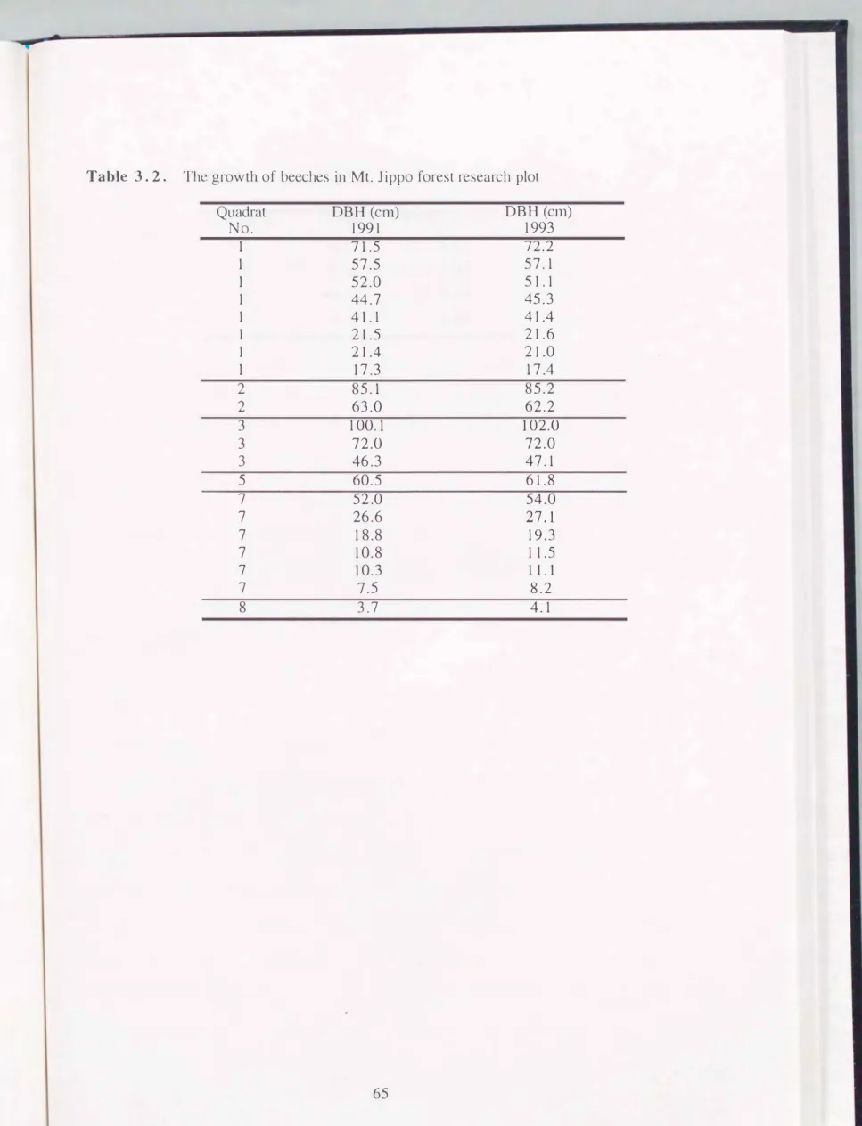
III. Sustainability of an Isolated Beech-Dwarf Bamboo Stand: Analysis of Forest Dynamics with Individual Based Model 3 .1. Introduction ..^{. . . . .}.^...^....^{. . . .}.^..^{. . .}..^{. . .}.^..^..^{. . .}.^{. .}..^{. . . .}.^{. .}......^{. .}... . . ..^..^{. .}...^{. .} 38

3.2. Study area ^..^{. . .}.^..^{. .}..^... . . ..^...^{. . .}...^....^{. . . .}......^...^..^{. .}..^{. .}.^...^..^....^{. . . . .}. 39

3.3. Modelling and parameter estimation .... . . .... . . . ..^{. .}..^..^..^{. . . . .}.^...^....^{. .}...^..^...^{. 40}

3.4. Results .^{. .}....^...^..^..^...^....^... . . ...^{. .}..^.....^{. .}...^{. . .}.^{. .}.^{. . .}..^{. . . . .}.^{. .}...^....^..^{. . .}...^.. 47

3. 5. Discussion and conclusions .^..^...^{. .}.^{. ..}.^...^{. .}._{. . . . .}......^{. .}... . . ..^..^{. . . .}.^..^{. .}.^{. .}... 50

Appendix E: Maximmn likelihood estimate of growth parameters . .....^.......^.....^{. .} 52

IV. Acknowledgments .^..^..^..^....^{. .}.^..^{. . . . .}..^...^{. . .}..^..^{. .}..^..^{. . . .}.^..^{. . . .}..^..^..^..^{. .}.. . . ...^{. .}..^{. .} 54

V. References . . . ..^....^{. . .}.^{. .}..^{. .}....^......^... . . ..^... . . ..^{... .}.^{. ..}.. . . ..^{. .}..^{. .}.^...^..^{. . ...} 55

VI. Tables . . . . ..^...^{. . .}... . . ... . . ..^{. .}.^..^..^...^..^{. . .}.^{. .}..^{. . .}..^{. .}....^...^..^....^..^{. . . . .}.......^{. . . .}.^. 63

VII. Figure Legends .... . . ..^{. . .}.^{. . . .}..^..^. .-... 67

I. Preface

In order to construct a mathematical model aiming to explain some ecological dynamics and patterns observed in the field, we should pay attention in two processes:

explicit paran1eterization based on field measurements and choosing the correct procedure for calculating the model. The purpose of this study is to investigate how we develop a model of forest dynamics realizing both of these points.

I would like to focus on the forest dynamics in the range of 0.01 to several decades hectors. In such scale, forest ecologists can track the time change of the size of all trees in a research plot, hence they consider the relationship between the forest dynanlics and its size structure (e. g. Nakashizuka et al., 1992). Here we review four major models to answer the problems in such spatial scale: JABOWA-FORET models, density distribution models de cribed by Fokker-Planck equation, SORTIE and lattice models of wave regeneration. All of them has two common features: considering the size structure in which the size of each tree is denoted by a real number and the localized interaction between individual trees. Let me briefly outline them in the following.

Forest simulators like J ABOW A (Botkin et al., 1972) and FORET (Shugart, 1984) are the most widely studied for the forest all over the world. Here we call them J ABOW A-FORET 1nodels. One of the feature of this series is that whole forest dynamics is represented as an ensemble of the small stands (or, patches) in which the fate of every tree are tracked. This approach is called individual based modeling. Although all the parameter was detern1ined based on field observation, the way of their paraineterization is not always cleaJ·. For example, Shugart (1984) classify the shade tolerance of trees in three categories, but there are no the statistical justification for such modeling. In addition, Pacala et aL. ( 1996) pointed out "the single greatest shortcoming"

of J ABOW A-FORET models was that they simply assign the same growth dependent mortality function to all specie because of the lack of published data relating growth and mortality. These things might suggest the importance of explicit parameterization.

In the second approach, the density distribution of trees is directly calculated by a partial differential equation. The density distribution is the function of time and the size of trees. Kohyama (1989, 1991, 1992a and 1992b) applied this method to explain the coexistence of trees observed in a warm-temperate rain forest in southern 1 apan dominated by evergreen broad trees, and found the tnechanism, called the architecture hypothesis, maintaining the species diversity of forest trees. Although such a new understanding was obtained and the method to estimate parameters are much more explicit that those of .TAB OW A-FORET models, it could be said that the assumption for calculation is not so realistic. The assun1ption, frequently called mean field approximation, is to set always the correlation between trees zero. Certainly, if there were no interaction between trees, the Fokker-Planck equation would work well.

However, the "one-directional competition" (explained in chapter III) i significantly detected in the field (e.g. Kohyama, 1992a). Hence it is natural that such the local competition generate the forest with negative covariance structure, or in other tenns, the forest becomes mosaic-like structure of two different kind of patches, one where a few large canopy trees suppress the newly settlement of small trees and the other called

"canopy gap" with a large number of small trees and no canopy tree. It can be said that the mean field approxin1ation encounters difficulties to calculate the forest dynamics with local; interaction and local disturbance.

Recently, Kohyama ( 1993 and 1994) developed a improved model to avoid the prohlem by introducing a new dimension, "patch age" to separate the old mature patches from "young" (i.e. canopy gaps). This technique succeeded to generate the negative covariance structure in forest, however, the modification of the mean approximation would face a new difficulty: the age of a patch is defined as the passing time from the last disturbance de troying the patch, and it is very hard to measure the accurate value of such the "age" in the field.

One of the modern forest simulator, SORTIE (Pacala et al., 1993 and 1996) has

realized an ideal synthesis of explicit parameterization (maxitnum likelihood method) and appropriate calculation (individual based modeling). The SORTIE is an empirically based model of forest dynamics derived from data in the research plot in Connecticut, USA. It tracks the position of each tree and determines tree performance based on the individual's local neighborhood. Pacala and his colleague revealed the importance of spatial structure in forest dynamics and the functional responses of forest against various disturbances. We have only one practical difficulty in SORTIE: it needs much more power of computer than JABOW A-FORET models.

Constructing more simple and abstract model than those in above, lattice struCLLired models (lwasa et al., 1991� Sato and Iwasa, 1993) succeeded to generate the wave-like regeneration pattern observed on subalpine forests. In these ·models, whole forest con i ts of a large number of sites arrayed on one or two dimensional rectangular lattice. A site is assumed that a cohort of trees. The interaction between sites is always local and horizontally one-directional. Most of its parameters are estimated from field data, and a few unknown are determined such that the generated pattern of tree height becmnes similar to that in the real forest.

In this thesis, I investigate two models for forest dynamics with considering the merits and demerits of the model in above. In chapter II, I develop a simple lattice model which has only two states (gap and nongap) for each site. This model was deve!l>ped to predict the forest canopy dynamics with localized interaction between sites.

The importance of local correlation is shown by comparing the results from the mean field approximation (in this case, mean field of horizontal space) and the pair approximation which calculates the approximated correlation between two neighbor sites. Because this study aims to understand how processes at local scale are translates into patterns at larger scale, the global statistics like mean local density or gap size distribution are examined by comparing to the indexes measured i·n Barro Colorado Island, Panama.

In chapter III, ^an individual based rnodel is developed to evaluate the sustainability of an isolated beech stand with Sasa undergrowth which disappears and recovers reciprocally. The basic design of this model is similar to that of JABOWA­

FORET models, while the submodel of growth is almost the same ^a5 that of Kohyama' s model. The pa.ran1eters used in the subtnodel are estimated by using maximum likelihood rr1ethod like SORTIE. The sustainability of an isolated beech starld is evaluated by a statistical index calculated from several hundreds of replications of simulation.

In the following, I summarize the content of each chapter in more detail.

Chapter II. Forest Spatial Dynamics with Gap Expansion: Total Gap Area and Gap Size Distribution

Recent studies on forest dynamics in diverse forested ecosystems suggest that forest stands are disturbed more frequently if they are next to existing gaps, and that gaps once forn1ed tend to expand their area in subsequent years. We examine total gap area and the size distribution of gaps at equilibrium in a lattice structured forest model. Each site undergoes transition between two states (gaps and nongaps), and the disturbance rate (tran. iLion from nongap to gap) increases with the number of gap sites in the neighborhood. Dynamics based on mean-field approximation (i.e. neglecting of spatial structure) failed to predict total gap area and the gap size distribution in the equilibrium foresl. Pair approximation, which considers in a closed dynan1ical system of average and local gap density (the conditional gap density among neighbors of a randomly chosen gap site), can predict the total gap area, the correlation between neighbors, and the gap size distribution fairly accurately. If the recruitment rate increases in proportion to nongap ^a.rcel in the forest, the model may show bistability. We analyze data on forest spatial dynan1ics in the light of the model. We conclude that gap size distribution can

often be described using two statistics (global and local gap densities) and that these in turn can be predicted by the dynamics of gap formation, gap expansion, regeneration, and gap closure.

Chapter III. Sustainability of an Isolated Beech-Dwarf Bamboo Stand: Analysis of Forest Dynamics with Individual Based Model

The beech Fagus crenata forest on Mt. Jippo in southwestern Japan has been diminished in stnall fragn1ents by past human activity. The forest floor is covered by dense dwarf bamboo, Sasa, which is an inhibitor of beech regeneration. One of the ecolo�ical feature of Sasa is that they wither synchronously over a large area once in several decades. An individual based model (IBM) was developed to evaluate the sustainability of such a fragmented beech stand with considering the dynamics of Sasa.

The model has three submodels for beech individuals: growth, mortality and seed production. The parameters of these submodels are estimated from field measurements.

By using this model together with Sasa dynamics, we can evaluate the adverse effect of Sasa on enhancing the risk of extinction of a single fragmented beech stand during 500 years. The results obtained by Monte Carlo simulations are: ( l) Sasa has a strong in1pact on the sustainability of a isolated beech stand; (2) The effects of two parameters for Sasa life history, the longevity and the recovery titne, can be statistically separated from each other; and (3) The probability of extinction of a beech stand depends much more ��trongly on the parameters of beech mortality than those of growth rate.

II. Forest Spatial Dynamics with Gap Expansion:

Total Gap Area and Gap Size Distribution·

2.1. Introduction

Last two decades, many ecologists working on forest dynamics have focused their attention to "gaps", openings created in the forest canopy (Whitmore, 1975; _Yamamoto, 1992).

Gaps tnay range in area from the openings created by the death of a single branch to larger scale blowdown of a catastrophic disturbance, such as a storm, a fire or an aggregated insect outbreak. The size, the number and the spatial distribution of gaps and the processes of gap formation and canopy recovery have been studied extensively (e.g. Kanzaki et al., 1994;

Nakashizuka, 1987, 1991; _Runkle, 1984; Yan1amoto, 1992, 1993; _Masaki etal., 1992).

Many studies of forest gap dynamics have demonstrated that new gaps are more likely to occur adjacent to pre-existing gaps. Trees in the border of gaps tend to have a higher rate of disturbances.

For example, Foster and Reiners ( 1986) reported the size distribution and expansion of canopy gaps in a subalpine spruce-fir forest in the White Mountains, USA. The gap area distribution was a negative exponential in forn1. They observed that gap expansion occurs as the result of the fall of canopy trees at gap perimeters subsequent to initial gap formation. By the gap expansion process, the areas of gaps were increased from the initial value by factors of 1.4 _to 13.7. Since wind was the n1ajor gap-fonning disturbance agent, the increased

exposure to wind of trees at gap edges suggested that wind-induced treefall were continuously eroding the 1nargins of gaps. A similar expansion of gaps was also reported in a subalpine forest in Japan: Kamiyama and Ohnishi (1981) analyzed aerial photographs in different years:

1948, 1959, 1969, _and 1979. _{For example,} a gap, which was absent on a photograph taken in 1948, appeared first in 1959 and expanded toward all the directions during subsequent 20

• Thi, chapter was done in collaboration with Prof. Yoh Iwasa and Mr. Naoki Furumoto.

years. Foresters have long been aware of the increased incidence of wind throw at the downwind edges of logging-created forest openings in spruce-fir forest (Alexander, 1964 ).

In an old-growth deciduous forest, Runkle (1984) recensused canopy gaps 4 _year following his initial census and found that 11 o/o of the gaps had enlarged by the blowdown on peripheral canopy trees, and that 31% of the gaps had enlarged via the death standing of surrounding trees, but the mortality of gap-edge trees was the same as for overstory trees in general.

[n a wind-exposed tropical cloud forest in Costa Rica, Lawton and Putz ( 1988) _found gaps spatially aggregated, with more gaps occurring within 17-20 m of one another than expected by chance. Kanzaki et al. ( 1994) observed in tropical seasonal evergreen forest in Thailand that all the gaps formed fr01n 1985 _to 1993 in their belt plot were in contact with older gaps or building-phase patches (low in height).

A very clear quantitative demonstration of new gap formation occurring near pre­

existing gaps was given by Hubbell and Foster ( 1986) from their study of Panamanian neotropical forests. They observed that trees adjacent to gaps, or trees standing above the surrounding canopy, suffer a greater risk of falling than trees which are surrounded by plants as tall or taller than themselves. The analysis of spatial patterns of trees in 1983 _{and in} 1984 showed that drops in canopy height are much more likely to occur on the edges of gaps. The data were arranged on a regular two-dimensional square lattice with each unit a 5x5 _{m plot}

(we call this a 'site' in the following). If the focal plot in the centre was taller than 30m in 1983, and all neighboring plots were taller than 30m as well, the probability of a fall in canopy height in the focal plot to lower class in a year was only 0.039. In contrast, focal plots

surrounded by all 8 neighboring plots less than 20 m height had an annual rate of fall of 50o/o (0.515).

Another very clear example of enhanced disturbance rate by the surrounding neighbors with lower height is given by wave regeneration, fir-wave, or Shimagare in Japanese (Sprugel, 1976� _Kohyan1a, 1988� Kohyama and Fujita, 1981): In subalpine forests dominated by Abies

species in Japan and Northeast USA, forests show a large scaled regeneration pattern with many stripes of stand-level dieback perpendicular to the direction of prevailing wind, spaced regularly with the distance between adjacent die back zones of about

100-150

m, with the whole pattern 1noving slowly

(1-1.5

m per year) downwind.

In a lattice structured model in which each site is a forest stand occupied by a cohort of trees, it has been shown that simple rules of mortality and growth are capable of generating regular wave-regenerating pattern fron1 random initial patterns if the trees much taller than windward neighboring sites die after some number of years (I was a et al.,

1991;

_{Sato and}

Iwasa,

1993).

Comparing the n1odel with the observed data of canopy height, growth rate, and the speed of waves, we can predict parameters difficult to measure directly, such as the time required for newly exposed cohort of trees to show stand level dieback and the spatial range of wind-shielding effect (lwasa ^et al.,

1991

₎

.

A very useful Inethod of modelling when the interaction between neighbors is important is lattice st1uctured models, or cellular automata models, which consider the nearest neighbor interaction explicitly. Models for wave regeneration (Iwasa ^et al.,

1991;

Sato and Iwasa,

1993)

are examples of the use of lattice models in forest dynarnics. Other examples of lattice

structured models in population biology include not only forest dynamics (Green,

1989;

Smith and Urban,

1988;

Nakashizuka,

1991;

Kawano and Iwasa,

1993),

but also population dyna1nics with perennials capable of vegetative propagation (Crawley and May,

1987;

Silvertown,

1992;

Harada and Iwasa,

1994),

marine invertebrate community (Caswell and Etter,

1992;

Etter and Caswell,

1994 )

, predator-prey (Tainaka,

1988;

_{de Roos et al.,}

1991;

Wilson eta/.,

1993 ),

host-pathogen (Ohtsuki and Keyes,

1986;

_{Sa to et al.,}

1994

), and host­

parasitoid (Hassell eta/.,

1991, 1994)

dynamics with spatial structure.

Jn this paper, we examine the effect of gap expansion on total gap area and the size di tribution of gaps in lattice structured population models. The forest is assumed to be composed of many sites arranged on a regular square lattice, each corresponding to a forest stand of about

1

_Ox

10

_In. Each ite is either a gap or a nongap, and changes its state between

the two stochastically. The rate of disturbance, causing a transition from a non gap site to a gap site would increase with the number of neighbors which are currently in gap state, indicating gap expansion. We analyze the model by three methods: ( 1) mean-field

approximation (ignoring spatial structure), (2) pair-approximation (tracing both the average gap density and the correlation between neighbors), and (3) computer simulation.

Pair approxi1nation is a technique which constructs the simultaneous dynamics of the average density and the neighbor-conditional local density by neglecting correlation beyond nearest neighbors. It has been shown to be very powerful for analyzing the population

dynamics with spatial structure although it is not exact (Matsuda ^et al., 1992; _{Sa to} eta!., 1994;

Harada and Iwasa, 1994; _{Harada et} al., 1995). Because of gap expansion, spatial pattern of gap sites generated by the model is aggregated, forming more large gap clusters than expected by chance in a random spatial pattern. We construct a closed dynamical system for the global density of gap sites (total fraction of gap sites in the syste1n) and the local density of gap sites (the fraction of gap sites among neighbors of gap sites), the latter being larger than the former due to spatial clLilnping. We conclude that gap size distribution can often be smrunarize by two statistics (global and local gap densities) and that these can be predicted from the processes of gap formation, gap expansion, regeneration and gap closure.

2.2. Model

We consider a habitat consisting of infinitely many sites arranged on a regular lattice.

Each lattice site corresponds to a forest stand of area about 1 Q.r. 10 m and can be occupied by a large canopy tree.

After canopy trees fall due to disturbances of various sources, the site becomes a "gap"

site. It takes some number of years until young trees from seedlings or seeds will grow and fill the gap. During this recovering period, the height of trees is still clearly lower than the height of surrounding mature canopy trees, and can be recognized as a gap. In general, we may classify the state of a site into a gap phase, a building phase and a mature phase (Whitmore,

1975; Kanzaki etal., 1994), or lo several size categories (Hubbell and Foster, 1986). Here we simply consider two categories only: gaps and nongaps. An operational definition of gaps and nongaps is given by choosing a certain threshold height, say 20 m (Runkle, 1984; Hubbell and Foster, 1986), 10 n1 (Runkle, 1981; Yamamoto, 1993), or 3 m (Lawton and Putz, 1988), depending on the height of mature canopy trees, and regarding a site as a gap site if the height of trees is lower than that level.

Transition fr01n a newly formed gap to a nongap may occur by canopy closure, instead of growth by new recruiting individuals. For a single individual seedling to reach the canopy layer, n1ultiple gap episode may be needed (Runkle and Yetter, 1987). In this paper, we do not consider detailed mechanisms of canopy recovery, but we concentrate on the fraction and the spatial pattetn of gaps in the forests.

We denote a gap or a nongap by two symbols, 0 and+, respectively and assume that each site experiences transition between the two states through tin1e. Although real fo^rest^{s are} 2-dimensional, we examine both 1-ditnensional and 2-dimensional lattices in this paper.

Applying the analysis to !-dimensional system is useful in checking the accuracy of our

method of analysis in different situations, and also useful in explaining method of analysis, e.g.

calculating the frequency of gap cluster of a particular size. In addition, the effect" of spatial structure to population dynamics is n1ore pronounced in a !-dimensional model than in a 2- dimensional model.

Before examining the case in which gaps expand to adjacent occupied sites, we first sununarize the results for cases in which each site of the forest undergoes independent transition bet ween gap and non gap states: A gap site becomes a nongap by the growth of trees in the site, and a nongap site becomes a gap due to the death of canopy trees by

disturbances. Assmne that the rate of transition fron1 a gap to a non gap occur at rate b per year, and transition from a nongap to a gap occurs at rate d. The inverse of recruitment rate,

lib, is the average length of time for sites to be gaps (recovery time), and the inverse of

disturbance rate, 1/d, is the average length of time for sites to be nongaps (average tenure of canopy trees).

b

(0) (+)

d

The fraction of gap sites in the equilibrium is

d l(b+d ).

Gaps are distributed randomly over the lattice because different sites are independent of each other (Fig.

2.1

_A).

2.2.1. Gaps causing ^more gaps

The enhanced disturbance rate per site in the periphery of gaps is reported in subalpine spruce-fir forest (Lawton and Putz,

1988),

in deciduous old-growth forest (Runkle,

1984

_),

and in tropical forest (Hubbell and Foster,

1986;

_Kanzaki et al.,

1994).

Wave-regeneration of Abies forest (Kohyama,

1988;

_Sprugel,

1976)

is an illuminating example of large scaled pattern formed by between-stands interaction, in which a cohort of trees in a site experience a stand-level dieback if its windward neighbors are clearly shorter than the site.

As the simplest modeling of gap expansion, we consider the case in which the transition rate fro1n a nongap to a gap increases with the number of neighbors which are gaps. For example we assume that the transition rate is not a constant d but is an increasing function of the number of surrounding gap sites. Let ⁿ

(0)

be the number of

0

sites among the nearest neighbors. It satisfies

0 �

n

(0) � z,

_where

z

is the number of nearest neighbors:

z=2

_for a

one-dimensional linear lattice,

z=4

for a two-dimensional square lattice with Neumann neighborhood, and

z=8

for two-dimensional system with Moore neighborhood (Durrett and Levin,

1994). z

can be even larger if ecological interaction occurs between more distant

neighbors, such as

2

step neighbors. We assume that an individual with ⁿ

(0)

gap neighbors has the dealh rate d

+ 1i

₇ n

(0).

The rate of transition from a nongap site to a gap site is the highest when all the surrounding nearest neighbors are gaps and is equal to

d +

_6.

b

{0) (+)

d ⁺

�

₇ n

(0)

We assmne that each transition event occurs instantaneously at rates given above. The model then gives a continuous-time Markov chain (Liggett,

1985).

Starting from a random initial distribution, the spatial pattern would change with time, and becomes a clumped

distribution, as shown in Fig.

2.1B.

If spontaneous disturbance is absent, the model is called the basic contact process (Griffeath,

1979).

2.3. Total gap area

Now we consider the total gap area, or the fraction of gap sites in the equilibrium

forests. Let P+ be the fraction of nongap sites in the whole lattice, or the probability for a randomly chosen site to be occupied. Similarly let Po be the fraction of gap sites, or the probability for a randomly chosen site to be a gap. We may call these two quantities the global ciensities of states

+

^{and 0,} respectively (Matsuda ^et al.,

1992;

Harada and I was a,

1994 ).

They are the average densities of nongap sites and gap sites, respectively.

The dynamics of the total fraction of gap sites, or the global density Po, are :

d Po

( )

-1-_{( t} ⁼ -b Po

+ d +8

qo;+ P+

(2.1)

The first term in the right hand side indicates the transition from a gap site to a nongap site

(0-

>

+)

hy the recruitment and growth of trees. We here assume that the transition occurs

randomly at rate b. The second term of Eq. 2.1 indicates disturbances, causing transition from a nongap site to a gap site ( ^{+ ->}

0).

This te1111 includes both random creation of novel gaps independent of nearest neighbors at a rated, and the expansion of existing gaps towards their neighboring ites. To express this transition rate per nongap site, we need the

conditional probability that a randomly chosen neighbor of an occupied site (state+) is a gap (state 0). We denote this conditional probability by q0f+, which is an example of local

densities (Matsuda, 1987; Matsuda ^et al., 1992). Local densities like this indicate the degree of crowding around each individual or site, and q+l+ is closely related to the "mean

crowding" index ^m *(Lloyd, 1967) for clumping of spatial patterns (see Harada and Iwasa, 1994 ).

fn the following, we discuss two ways to derive the dynamics for gap density: one is a traditional way of neglecting spatial structure, and the other is pair approximation.

2.3.1. Mean-field approximation

A conm1on way to simplify population dynamics, such as Eq. 2.1, is just to neglect spatial structure. This can be done by neglecting the correlation between neighbors, i.e. by assuming that the local density is the same as the global density: q

o

;o ⁼ qo;+ ⁼

Po

. If we adopt this simplification, the dynamics of the global density Po given by Eq. 2.1 are:

�!_Po

_dt

=

_d -

{

b +d

-8 ⁽

¹

^{-Po)} P}

^{o (2.2)}

where we used relation

P

+

=

^{1 -po.} Eq. 2.2 gives an autonomous differential equation for

the global gap density Po . Standard analysis shows that Eq. 2.2 has a single globally stable equilibrium between 0 and 1, which is derived from dpo ldt ⁼ 0. The equilibrium fraction of gap area is:

Pit= -(b

^+d

-8)

⁺

Y(b

^+d

-8 f

^{+4d 8 (2.3)}

2

8

where superfix M indicates mean-field approximation. When

8 =

^0, this equilibrium becomes

p{t =

^_d__, the fraction of occupied sites in the case without interaction.

b+d

2.3.2. Pair approximation and clumped distribution

Instead of neglecting the difference between global and local density, we may

distinguish them and derive a closed dynamical system for both variables. Pair approximation is a method of constn1cting a system of ordinary differential equations for the global density

and the local density (Harada and Iwasa,

1994 ).

First we note that

qol+

⁼

( 1 - _qo!O)Pol( 1 _{- Po)}

holds from the definition of conditional probability. Using this relation, Eq.

2.1

is rewritten as

d Po {

}

-

dt

=

d- b _+d

_-8

₍ 1 -qo!O) Po

which gives the dynamics of global density

Po

in terms of local density

qo!O·

(2.4)

Since the

dynamics of global density

Po,

given by Eq.

2.4,

is determined by

Po

and

qoJo,

we must consider a differential equation for

qo!O·

^Let

Poo

be the density of

(0,0)

pairs, i.e. the probability for a randomly chosen nearest neighbors to be gap sites. According to the definition of conditional probability, the local density

qo1o

is equal to ratio

Pool po,

^{and hence}

the dynamics of local density are:

d _qo1o

=

_ _Poo d _Po + _1 d _Poo dt _p02 dt _Po dt

The time change of

Poo

^is:

li � _too

=

-2b _{Poo +} 2/d ₊

₀

_{(± + Y qot+O )} ) _P+o (2.5)

where the first ten11 indicates a transition of a

(0,0)

pair to a

( +,0)

_pair. Here we denote that

P+O

^is the probability that a randomly chos�n nearest neighbor pair is a

( +,0)

pair in this order, distinguishing the order of two sites. Factor

2

comes from the fact that the recruitment of

either of the two sites can turn

+

to make such a transition. The total fraction of pairs of+ and 0, neglecting the order, is hence 2P+O· The second term of Eq. 2.5 indicates a transition from a ( +,0) pair to a (0,0) pair. Here we note that the mortality depends on the fraction of 0 sites in nearest neighbors of a

+

site, where one of the nearest neighbor of the

+

site is known to be 0. In Eq. 2.5, we denote this higher order conditional probability by ^qoi+O·

The conditional probability ^qol+o can be expressed by using a still higher probability related to a triplet instead of a doublet, but the dynamics for triplet probabilities will include

conditiClnal probabilities of a still higher order. We here introduce a pair approximation, namely CJOI+O is replaced by ^{qo;+ =}

(

_{1 -qo;o)}

_E_Q_

(In general, ^{qald d'} is replaced by ^qa/d,

1 -Po

Matsuda eta/., 1992), in which the correlation beyond nearest neighbors is neglected.

Using Eq. 2.4 and Eq. 2.5 with the pair approximation, the dynamics of local gap density ^qo;o can be rewritten as:

dt Po

d

_qo;o = -qo;o

[_d__ -{b +d -8 (

_{1 -qo;o}

)} J

-2b qoto +2

(I

_-qo!O)

[ ^{d +8 (} +} <:.f ^(I

^-qoto)

/�

⁰

) ]

^(2.6)

Eqs. 2.4 and 2.6 constitute a closed dynamical system of two variables, p0 and qo10. Now

we apply standard analysis of nonlinear differential equations to these equations. The equilibrium of Eqs. 2.4 and 2.6 can be obtained from

d:o

^{= 0 and}

^d !�'0

^{= 0, as follows:}

") (b ^{+d +8 L±l )} -Y(b ^{+d +8}

^L±l

⁾

²

^-

⁴

⁸ (b ^{+ a.+ �)}

l/1 _{0/0 -}- 1 -b ^{z z z z}

( ⁾

pp-

d

u -

5:

(

... p

)

b

+d

_{-u 1 -qo;o}

28 b 4 ⁺ �

where superfix P indicates pair approxin1ation.

(2.7a) (2.7b)

fn Appendix A, we can prove that in the lim.it when ^z increases infinitely large,

q[;10

and

Pb

^{in Eqs.} 2.7a, 2.7b converge to

pf:

given by Eq. 2.3, the average gap density

predicted by mean-field approximation. A similar result has been proved rigorously ford= 0, the basic contact process (Bramson ^et al., 1989). This implies that when the range of

ecological interactions is large and includes tnany sites, the dynamics become similar to the case of con1plete n1ixing.

ln the absence of interaction between neighbors ( o = 0), the equilibrium local density and the global density predicted by pair approximation are both equal to _d_.

h+d

In Appendix A, we prove that local gap density is greater than the global gap density

(qb;o

^>

(>�)

^{if o > 0.} We also prove that the density predicted by mean-field approximation is between these two densities predicted by pair approximation

(p{;

^<

p[)1

^<

_qb10).

The global and local densities for nongap sites are calculated from

P6

and

q _b10

^:

p l ^p

P+

^{= -}

P _o

qfl+

= 1 -

(

¹

- qb!O)p(;�

1

- P6)

[n this section, we first constructed the dynamics of

Po

and

qo10,

the global and the

local densities of gap sites based on pair approximation, and then from the equilibrium, we predict:

P+

and q+f+, the global and the local densities of nongap sites. Alternatively, we may start with the dynamics of global and local densities of nongap sites

P+

and q+f+, based

on pair approximation, and then calculate

Po

^and

qo1o

from these result . This is done in Appendix B. Calculation is ^a little easier than the one in this section, but the result is almost exactly the same.

2.4. Computer simulation

In order to know the accuracy of the two methods of constructing approxin1ated population dynamics (mean-field approximation and pair approximation), we con1pare the predictions of these dynamics with the direct computer simulation. We examine both one­

dimensional and two-dimensional systems. Since the results of one-dimensional system ^are more pronounced than those of two-dimensional system, we first explain the former.

2.4.1. One-dimensional system

Stands are arranged on a circular lattice including about 1000 sites. To remove the effect of edges, we assume periodic boundary condition. In the initial pattern, each site is a gap or ^a nongap independently with a constant probability. After 1000 tin1e units, the spatial pattern reaches to the equilibrium and the fraction of gap sites

Po

and the conditional fraction of gap sites among neighbors of gaps

q010

are stabilized, and then they fluctuate with small amplituJe around their means due to the finiteness of the total number of sites. To remove these small fluctuation, we calculate the average density of gaps over many generations after the equilibrium is reached.

Figure 2.2A illustrates the equilibrium global density

Po

and local density

qo;o

for different 8, the neighbor-dependent mortality. We used b = 0.20, implying that the average gap age is 5 tin1e units. The death rate caused by neighbor-independent component of disturbance is d = 0.01, which indicates the average tenure for canopy trees in the middle of continuous canopy is 100 time units. Symbols in this figure are the results of computer simulation: Solid circles are for global gap density

Po

, and triangles are for local gap density

qo1o.

The local density of gaps is significantly higher than the global density, indicating a clumped spatial distribution of gap sites.

Mean field approximation does not distinguish these two densities, and its prediction

pfrl

is shown by a broken line. In the mean-field approximation, the equilibrium of local density1

qtl)0,

is the same as the global density

pfrl,

which is not the ca e for computer simulation.

The solid curve is for

p6,

and the gray one is for

q{;10,

given by Eq. 2.7a and 2.7b,

respectively with ^{z =} 2. Prediction by pair approximation is clearly more accurate than that by mean-field approximation, and pair approximation correctly predicts that

qo;o

is larger than

po.

We can see that the gap density given by mean-field approximation is larger than the global density given by pair approximation but smaller than the local density given by the pair approxirnation.

In Fig. 2.2A, we also indicated the global density

P+

by open circles and the local density (}+!+of nongap sites by squares. The local density is clearly higher than the global density, i1nplying that the spatial pattern of non gap sites is also clumped. Predictions based on pair approximation are given by solid curves, which are quite accurate.

2.4.2. Two-dimensional system

'N e also conducted the simulation in a two-dimensional system on a 1 QQJ.l 00 lattice with periodic boundary condition (a torus type). Fig. 2.2B illustrates the results.

Parameters are the same as in Fig. 2.2A.

Solid lines are the average fractions of gap sites

P6

and the fractions of gap sites among neighbors of randomly chosen gap sites

q610,

given by Eqs. 2.7a and 2.7b with ^{z =} 4, derived based on pair approximation. These lines fit very well the results of computer simulation shown by solid circles. A broken line is the prediction by mean-field approximation Eq. 2.3 with ^{z =} 4. It overestimates the fraction of gap sites.

'T'hese results are qualitatively the same as in one-dimensional system, but the difference between different n1ethods of approximation is less pronounced in two-dimensional case than in one-dimensional case (Fig. 2.2A).

2.5. Supply-dependent recruitment and bistability

So far, we have assumed that seeds or seedlings needed for recruitment are always available and the rate of transition from newly formed gaps to nongaps is independent of the

number of parent trees that supply seeds. We may consider the case in which the supply of recruit1nent is strongly limiting the recovery process.

To simplify the situation, we here examine two cases: [ 1] recovery rate of a gap is proportional to the number of nongap sites in the forest, and [2] it is proportional to the number of nongap sites in the neighbors.

2.5 .1. Recovery proportional to global density of non gap sites

First, we consider the case in which the recovery rate of a gap site is proportional to the fraction of nongap sites in the whole forest, so that b is replaced by ap+, where a _is a positive constant. The equilibria of the dynamics based on the mean-field approximation and of those based on the pair approximation are shown in Appendix C. We see that there is a parameter region in which there are two simultaneously stable equilibria: one is for the positive

equilibrium with a sufficiently high density and the other with Po = _1, implying the absence of trees.

Figure 2.3A illustrates the equilibrium global density Po and local density qo;o for different neighbor-dependent mortality 8 for one-di1nensional system. We fixed other parameters (a= 0.20, _d = 0.01 )_. Circles are the results from computer simulation. Solid circles are for the global density po, and triangles are for local density qo;o. The result from mean field approximation is shown by a broken line. Solid curve is global gap density

Pb,

and gray one is local gap density

qg10,

Eq. C3 with ^{z =} 2. Prediction by pair approximation is more accurate that by mean field approximation, and pair approximation correctly predicts that qo;o is larger than po.

We also conducted the simulation of a two-dimensional system on a 100.I.100 _lattice with periodic boundary condition (torus type). Fig. 2.3B illustrates the case of two­

dimensional system with theoretical curves, Eq. C3 with ^{z =} 4. We observe the same tendency as for one-dimensional circular lattice 1nodel, but the differences between curves are less pronounced than in one-dimensional system.

2 . 5. 2. Recovery proportional to local density of non gap sites

Next we consider the case in which recovery rate is proportional to the fraction of nongap sites in the neighborhood

(f3q+10).

This n1ay be the case in which the supply of the seeds or seedlings is possible only within a short distance, i.e. only to the nearest neighbors, implying relatively heavy seeds (e.g. acorn) with lirruted dispersal or vegetative propagation.

Analyses sin1ilar to the last section apply to this case, as shown in Appendix C. The results are illustrated in Fig. 2.3C, where bistability is not predicted by the pair approximation, nor is observed in computer simulation. The mean-field approximation gives

p()'l

that happens to be the same as

q610

(gray line).

Even if the recovery rate may depend on the global and local densities, it may not be directly proportional. In general, we need to exan1ine a nonlinear function of these densities.

A simplest generalization would be a sum of three terms: a term independent of the parents, a term proportional to the fraction of nongap sites over the forests, and a term proportional to the number of nongap sites in the neighbors, as we will discuss later in the data analysis.

2.6. Gap size distribution

Now we consider the size distribution of gaps. The total gap area is the same between in Figs. 1 A and 1 B, but the spatial pattern of the gap sites is more clumped in Fig. 2.1 B than in Fig. 2. J A. Fig. 2. 1 B includes fewer and larger gaps than in Fig. 2.1 _A. Here and in the rest

of the paper, we regard a cluster of adjacent gap sites as a single large gap, and we call the number of sites included in a cluster of gap sites "the size of a gap" (Fig. 2.4 ).

2. 6.1. One-dimensional system

We begin with one-dimensional habitat in which each site has just two neighbors. Let k be the cluster size (or gap size), or the number of sites included a single cluster (or a gap).

Let ^nk be the number of clusters (gaps) of size k within a large area including lattice sites L.

Now the number of gap sites included in a cluster of size k is knk and the probability that a randon1ly chosen site is a member of cluster of size k is knk/ ^L.

First, consider the si1nplest case in which the spatial pattern is random. Those sites are either gap or nongap independently with probability Po and 1 - po, respectively. Then

the size of gaps follows a geo1netric distribution. To be specific, the probability that a particular site is included in a gap of size k is k Pok( 1 - po)2.

In the population with clumped distribution, the (unconditional) probability of a site to

be a gap site is different from the conditional probability that a nearest neighbor of a gap site is also a gap site. The latter is qo;o, which is larger than po. Pair approximation considers this difference but neglecting the correlation beyond nearest neighbors. Using this

approximation, we can express the probability of a randonliy chosen site is included in a cluster of size k as follows:

This was derived by the following consideration: First a randomly chosen site is a gap site with probability po. Second, the probability that x consecutive sites in the left and the k-1-x consecutive sites in the right of it are also a gap site and that the two surrounding sites for these k consecutive sites are nongaps is (q010f-1(1 - q010)2. Finally, there are k possible values for

x. The total fraction of gap sites is given by the sum of Eq. 2.8 over krJ I, and is equal to p0.

The number of gaps of size k in the whole lattice is:

(2.9)

We may compare the prediction of Eq. 2.9 with the gap size distribution obtained from computer sin1ulation. The equation has two parameters: the average fraction of gap site (Po )

and the fraction of gap sites among nearest neighbors of gaps (q010), which can be obtained

from the spatial pattern. Solid circles in Fig. 2.5 indicate the gap size distribution for the spatial patten1 generated by c01nputer simulations. Solid lines indicate the prediction given by Eq. 2.9 using two parameters

(po

,

qo;o)

estimated from the observed spatial pattern. They are quite accurate in predicting the result of computer simulations. This indicates the

usefulness of the approximation based on the neglect of higher order correlation beyond pairs.

ln Fig. 2.5, we also illustrated a gray line indicating the equation in which

qo;o

replaced by

Po·

This gray line is the gap-cluster distribution for the pattern generated by a random spatial pattern of the same total gap area. When interaction term is absent (8 ⁼ 0), the spatial pattern is random, and the broken and solid lines are the same. But for the cases with nearest neighbor interaction

(

8 ^> 0), we have fewer small clusters and more large clusters than predicted by random spatial pattern (gray curves) due to a clumped spatial distribution of gap

sites.

The broken line in Fig. 2.5 is the prediction using two parameters,

qo;o

and

po,

fron1 the pair approximation, Eqs. 2.7a and 2.7b. Here

qo;o

and

Po

are not from fitting to the data, but are calculated directly from basic parameters b, d, and 8 using the dynamics analyzed in a previous section. We can see that the prediction is fairly accurate, and that pair approximation can explain the gap size distribution very well without relying on the fitting procedures.

2.6.2. Two-dimensional system

Sin1ilarly, we can calculate the gap size distribution on regular two-dimensional square lattice for Neumann neighborhood, but computation is more complicated than the case for one­

dimensional systen1. For example, consider the probability that a randomly chosen site is an

isolated gap site, i.e. it is itself a single cluster of size 1. According to the spirit of pair approximation, it is simply

Po(

1 ^-

qo10)4,

where the site is a gap with probability p0 and all of it four neighbor are nongaps with conditional probability

(I - q010)4

(considering nearest neighbor correlation only). A sin1ilar probability for cluster of size 2 is

4p0q01J...l - q010)6,

where factor 4 comes from the number of configurations, and power 6 indicates the number of neighbors surrounding a (0,0)-pair.

Si1nilar consideration applies to ^a larger cluster size. Consider a gap site that belongs to a cluster of size k. Let

ck

be the total number of configurations of clusters of size k. We indicate the ith configuration among ck possibilities by

(i,

k). Let P(i,k) be the number of sites in the perimeter of the configuration (i, k). Then, based on the approximation neglecting higher order correlation beyond nearest neighbor pairs, the probability that a single site is included in a cluster of k-gaps is:

(2.10)

For one-dimensional case, Eq. 2.10 becomes Eq. 2.8 by using

ck

= k and P(i,k) = 2.

Table 2.l shows the perimeter polynomials of the two-dimensional site problem, f[x],

Ck

which is defined as f[x]

=-} ^I.

^{( 1 -}

^x)f(i,k).

We can rewrite Eq. 2.10 as follows:

i=

I

which gives the number of gaps of size k in a large area including L sites. These polynomials have been derived in physics, because the current model becomes site percolation process if sites are independent (Po= q01o) (Stauffer, 1985; Sykes and Glen, 1983).

Fig. 2.6 illustrates gap size distribution from the simulation model and the prediction by the equations above. Solid circles indicate the results from computer simulations. A solid line indicates the prediction given by Eq. 2.10 using two parameters estimated from the spatial pattern generated by computer simulation. They are quite accurate, again confirming the usefulness of the approximation of neglecting higher order correlation beyond pairs. Gray lines in Fig. 2.6 illustrate the equation given by Eq. 2.10 with qo1o replaced by p0. The

broken lines in Fig. 2.6 are the prediction using two paran1eters, qo;o and Po, from the dynamics based on pair approximation (Eqs. 2.7a and 2.7b). They are very close to the solid lines and are able to predict simulation results (solid circles).

Ln short, Eq. 2.10 with Eq. 2.7, based on pair approximation predict the cluster size (or gap size) distribution very accurately, both in one-dimensional and two-dimensional systems.

2.7. Discussion

Many successful computer models of forest dynamics assume that the forest is an ensen1ble of independent patches or stands (e.g. Botkin et al., 1972; Shugart, 1984; Leemans and Prentice, 1987; Kienast and Kuhn, 1989; Keane et al., 1990; Prentice and Lee mans, 1990;

Mohren and Kienast, 1991). In addition, an analysis of forest dynamics most frequently adopted is the use of a transition matrix, in which the state of forest stands is classified into several categories, according to canopy height (e.g. Hubbell and Foster, 1986) or to species con1po�;ition (Horn, 1974, 1975), and from the transition between one census to the next, the fractions of sites that undergo transition froin one category to another are estimated and summarized as a table (e.g. Caswell, 1989). Using this table of transition probability,

assuming Markovian property (neglect of past history), we can predict the temporal change and the equilibtimn composition of the forests.

However, we 1nust note that this method is valid only when we can neglect the interaction between nearest neighboring sites. As we have shown in this paper, interaction between neighboring sites, in a forrn of gap expansion, has profound effects on the spatial pattern, and subsequently on the forest dynamics.

In this paper we studied the total gap area and gap size distribution in a lattice structured

model in which disturbance occurs at a higher rate in nongap stands next to existing gaps than those surrounded by continuous canopy. Due to the neighbor-dependent mortality (8 _{> 0),} spatial distribution of gap sites becomes clumped (Fig. 2.1 B). The fraction of gap sites among neighbors of gap sites is significantly higher than the average fraction of gap sites

(qo;o > po). This clumped spatial distribution affects the equilibrium level of total gap area.

The dynamics based on mean-field approximation (neglecting nearest neighbor correlation) overestimate the equilibrium gap area, as shown by broken lines of Figs. 2A, 2B _and 3.

This is because the same total gap area would disturb the forest more extensively if it would be scattered over the forest with many more gap clusters. Spatial clumping of gap sites reduces the number of sites next to existing gap and the average rate of disturbance, and thus lowers a gap area level than predicted by the computation assuming random spatial distribution with the same total gap area (mean-field approximation).

In the case of supply-dependent recruitment illustrated in Fig. 2.3, the model may have simultaneously a locally stable positive equilibrium and a trivial equilibrium when trees are absent. This bistable situation can be predicted accurately by pair approximation but not by the mean-field approximation.

The pair approximation method constructs a closed dynamical system using average fraction of gap sites and the conditional fraction of gap sites among nearest neighbors of gaps, called global density and local density of gap sites, respectively. In a spatially structured model for herbaceous plants with vegetative reproduction and seed production, Harada and Iwasa ( 1994) showed that the local density is the same as the mean crowding by Lloyd ( 1967) if a sampling quadrat includes only a neighboring pair of sites. Mean crowding is defined as the average density experienced by individuals and has been developed as a very useful method of statistical analysis of spatial distribution (I wao, 1968; I wao and Kuno, 1971; Taylor, 1984;

lwasa and Teramoto, 1977, 1984 ). In the present mode, therefore, Po is the average gap density anJ qo1o the mean crowding of gap sites, and the dynamics of Eqs. 2.4 and 2.6 give closed autonomous equations for average density and mean crowding. The ratio of mean crowding to average density (denoted by m *1m) is called as patchiness index (lwao, 1968).

The ratio (jo;ol Po corresponds to the patchiness (the ratio of mean crowding to the mean density, denoted by m*lm) _(Iwao, 1968).

'In this paper, we also examined the size distribution of clusters of gap sites, or the size distribul ion of gaps if we regard a cluster of gap sites as a single large gap. The pair

approximation in spite of simple assumptions again gives an accurate prediction of the gap size distribution for a highly clumped spatial distribution including a rnuch higher fraction of large clusters than expected by chance (see Fig. 2.5 and 6).

2. 7 .1. Application to data from a tropical forest

To illustrate the use the present results to forest data, we here attempt to analyze the data in Hubbell and Foster ( 1986) from a neotropical forest in Barra Colorado Island, Panama.

They chose 5x5 m as the size of each lattice site, and showed the spatial patten1 of these sites as a map (Hubbell and Foster, p. 88, Fig. 2.3.4). On this rnap, [1] the sites lower than 20 m in height in 1983 census, [2] the sites higher than 20 m in 1983 but became lower than 20 m in height in the 1984 census, and [3] those that ren1ain higher both in 1983 and 1984 census times, are displayed in different colors (the figure 2. caption included a typographical mistake known from comparing Table 3.1 of Hubbell and Foster, 1986). By reading the data from the map (except for unreadable leftmost colun1n and bottom row), we can calculate various statistics needed for the analysis. The data we used for our analysis is in Fig. 2.7. By choosing 20 mas the lhreshold vegetation height separating gaps fron1 nongaps, the global gap density is Po= 0.331 and local gap density is qo;o = 0.580, and others are: q+l+ = 0.801,

qo;+ ⁼ 0. 199, and q+IO = 0.420, from the census in 1983. The spatial pattern is clumped, as qo;o >Po·

'l he transition rate of a nongap (taller than 20 m) to a gap (shorter than 20 m) increases with the numher of gap surrounding it in 1983 (Fig. 2.7). We attempted both Neumann neighborhood (z = 4) and Moore neighborhood (z = 8), and both gave very good fits to straight lines(Fig. 2.8). Since Neumann neighborhood gave a better fitting according to the likelihood function explained in Appendix 0, we use Neumann neighborhood for the analysis below.

A transition matrix (Table 3.1, p. 87, in Hubbell and Foster, 1986) shows that the one­

year transition of trees less than 20 m to taller than 20 m in the following year was b

=

^0.177

(=

1173/6631). In the model, the average transition rate from a nongap to a gap (disturbance rate) is d ⁺

8qo;o,

the parameters of which are known from the regression line

(z =

1) in Fig.

2.8, as d

=

^0.024 and

8

= 0.276.

We examine three models differing in the assumption of recovery process:

[Case

1]

Constant recovery rate:

Using the parameter b ⁼ 0.177, we can apply the model and the mean field

approximation predicts the equilibrium fraction of gap sites

Pt: ⁼

^0.461, which does not

explain the observed difference between global and local densities. Pair approximation gives the global density

Pb) =

^0.408 and the local density

qtro =

^0.485 at the equilibrium. These overestimate observed values:

Po=

^0.331 and

q

^o

¹

⁰

⁼

^0.580. In addition, their ratio

qb;dPS

^{= 1.189} is smaller than the observed

qo;oiPo

^{= 1. 752,} implying this model underestin1ates the patchiness of the spatial patterns.

[Case

2J

Recovery rate proportional to global density of nongap sites:

By setting 0.177

= ap+,

we can estimate

a=

^0.243. We may use the same parameters ford and

o

as in the last section. In this case, the dynamics based on pair approximation (Appendix C) predict the extinction of the whole population at the equilibrium:

P6 ⁼

^1. This does not fit to the observation.

[Case

3]

Recovery rate proportional to local density of nongap sites:

By setting 0.177

= f3q+;o,

we can estimate

f3 =

^0.423. Pair approximation in Appendix C predicts:

P6 ⁼

^{0.216 and}

^{q[;10 =}

^0.402. These underestimate the observed values for gap fractions. Their ratio is

q61of Pb ⁼

^1.861, implying a more clumped spatial distribution than the observed pattern.

In short, the observed values of global and local densities of gaps are in between the equilibrium in Case 1 (constant recovery rate) and that in Case 2 (recovery rate directly proportional to the local density of nongap sites). A sin1plest modelling in such a situation