解析的アプローチによるスラスタを用いた劣駆動衛星の位置・姿勢制御

(1)

九州大学学術情報リポジトリ

Kyushu University Institutional Repository

解析的アプローチによるスラスタを用いた劣駆動衛星の位置・姿勢制御

吉村, 康広

https://doi.org/10.15017/1398376

出版情報：Kyushu University, 2013, 博士（工学）, 課程博士バージョン：

権利関係：Fulltext available.

(2)

!

Doctoral Dissertation!

!

Analytical Approach to Position and Attitude Control of an Underactuated Satellite !

Using Thrusters!

!

解析的アプローチによるスラスタを用いた劣駆動衛星の位置・姿勢制御

!

Yasuhiro Yoshimura!

Kyushu University!

!

Supervisor: Professor Shinji Hokamoto!

!

September 2013

(3)

List of Figures

2.1 The existence region of the vector b. . . 12

2.2 The existence region of the vector T. . . 13

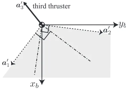
2.3 Third thruster allocation required for controllability. . . 14

2.4 The control torques formulated with three thrusters. . . 15

2.5 The control torque formulated with four thrusters . . . 16

2.6 Three-thruster configurations view from the positive zb-direction . . 19

2.7 The time histories of the angular velocity(asymmetric) . . . 20

2.8 The time histories of the wz-parameters(asymmetric) . . . 21

2.9 The time histories of the ZYX Euler angles(asymmetric) . . . 21

2.10 The time histories of the angular velocity(near-axisymmetric) . . . 22

2.11 The time histories of the wz-parameters(near-axisymmetric) . . . . 22

2.12 The time histories of the ZYX Euler angles(near-axisymmetric) . . 23

2.13 The time histories of the thruster forces in Fig. 2.6(a) . . . 23

2.14 The time histories of the thruster forces in Fig. 2.6(b) . . . 24

3.1 Thruster configuration. . . 28

3.2 Proposed control procedure with the invariant manifold in maneuver 3. . . 39

3.3 The proposed control procedure. . . 40

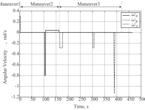
3.4 The time history of the angular velocity. . . 41

3.5 The time history of the attitude angle. . . 41

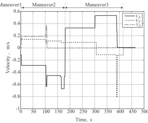
3.6 The time histories of the translational velocity. . . 42

3.7 The time history of the position. . . 42

3.8 Three-dimensional trajectory of the satellite. . . 43

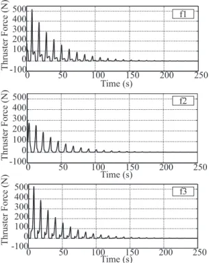
3.9 The time histories of the thruster inputs. . . 43

3.10 Lunar landing mission. . . 44

3.11 Satellite model . . . 45

3.12 Lunar lander model. . . 50

3.13 The relative error between the exact solution and the approximate solution. . . 51

3.14 Case2: The relative error between the exact solution and the approximate solution. . . 52

3.15 Control procedure for lunar landing mission. . . 54 1

(6)

3.16 The time history of translational velocity. . . 55

3.17 The time history of the satellite’s position. . . 56

3.18 The time histories of the control thrusts. . . 56

3.19 The time history of the satellite’s attitude angle. . . 57

3.20 The time history of the angular velocity. . . 58

4.1 Coordinate systems in formation flying. . . 62

4.3 Initial relative orbit . . . 69

4.4 Rendezvous maneuver using a drift motion. . . 71

4.5 The time history of follower position for the maneuver without attitude change. . . 72

4.6 The time history of LOS angle for the maneuver without attitude change. . . 73

4.7 The time histories of control thrusts for the maneuver without attitude change. . . 74

4.8 The time history of follower position for the proposed maneuver. . . 74

4.9 The time history of LOS angle for the proposed maneuver. . . 75

4.10 The time history of attitude angle of follower for the proposed maneuver. . . 75

4.11 The time histories of control thrusts for the proposed maneuver. . . 76

4.13 Attitude constraints in inertial frame . . . 80

4.14 Reconfiguration trajectory of the follower. . . 86

4.15 The time history of the attitude angle in inertial frame . . . 86

4.16 The input trajectory . . . 87

(7)

List of Tables

2.1 Simulation parameters . . . 19

3.1 Attitude control procedure. . . 30

3.2 Simulation Parameters. . . 39

3.3 Initial Conditions. . . 40

3.4 Satellite’s parameters. . . 51

3.5 Initial condition. . . 55

3.6 Simulation Results. . . 57

4.1 Simulation parameters . . . 71

4.2 Initial condition . . . 72

3

(8)

Chapter 1 Introduction

1.1 Background and Objective

Space probes require autonomous control to achieve their planetary explorations because of communication lag caused from large distance between the Earth and an asteroid or a planet. For example, the communication delay between a ground- station and the Near Earth Asteroid(NEA), Itokawa, which is located around 300 million kilometers away, is about 40 minutes [1]. Thus, in a proximity operation to an asteroid, a satellite firstly estimates the position and attitude of the satellite using several sensors, and then autonomously controls to a desired state using actuators, e.g., reaction wheels(RWs), control momentum gyros(CMGs), and thrusters. To this end, a large number of sensors and actuators are equipped on the satellite considering some of them as backup. Hayabusa, the first spacecraft achieved an asteroid sample return mission, had three RWs for attitude control and 12 chemical thrusters for both position and attitude control. These many actuators enable to generate translational forces independent from rotational torques and vice versa, and consequently it makes a control procedure much simple. If malfunctions of some actuators occur, however, the state control of the satellite becomes more complicated due to the coupling effect between the translation and the rotation. In such practical situation, the position and attitude control with the remained actuators is required to continue the mission. In other words, underactuated controllers have the possibility to extend satellite mission lifetimes.

Furthermore, from the viewpoint of a satellite design, the control method may be able to reduce the number of actuators equipped on the satellite even when considering some of them as backup.

When a nonlinear system has less number of inputs than the number of state variables, the system is called “underactuated” system. Since the number of inputs are limited, such system often includes nonintegrable constraints, i.e. “nonholonomic” constraints. It is known that control systems with nonholonomic constraints, called nonholonomic systems, have the possibility to control their state

(9)

variables in spite of the less number of inputs. Brockett [2] provides a necessary condition for symmetric affine systems, equivalently first-order nonholonomic systems, to be controllable. The condition indicates that no continuous state feedback can control the systems, and this negative result has motivated many researchers to derive nonholonomic control laws not to violate the condition. To avoid the Brockett’s condition, intensive studies have been conducted and consequently discontinuous controllers and time-varying feedback ones are proposed for symmetric affine systems [3–5]. The proposed methods can be applied to the systems described with a canonical form, whereas control theories for asymmetric affine systems have not been fully established.

This dissertation presents new control approaches for asymmetric affine systems, especially a satellite position and attitude control using a small number of thrusters. The control systems in this paper form a “second-order” nonholonomic system and have not only nonholonomic constraints due to a few thrusters, but also input constraints, i.e. the constant magnitudes of thrusts in one direction.

These input constraints thus disable to apply studies proposed on the second- order nonholonomic systems [6–8] to the systems in this dissertation, and even the controllability of the systems is hard to be discussed as shown in the following section. To tackle the problem, the control methods based on analytical solutions are proposed. The proposed methods would contribute to autonomous control of space probes in free-floating condition to continue the missions even when some actuators have failed and be useful to design backup systems of actuator configurations based on the underactuated controllers. Furthermore, the control method is extended to a control of formation flying of a satellite, a key technology for future space missions.

1.2 Literature Review

An attitude control of a satellite with less than three inputs is a nonholonomic system due to the angular momentum conservation. Crouch [9] provides necessary and sufficient conditions for an attitude control of an underactuated satellite considering RWs or pairs of gas-jet thrusters as actuators. The paper claims the pairs of gas-jet thrusters can control when the control torques are applied around two principal axes of the satellite, whereas less than three RWs cannot control the satellite attitude due to the angular momentum conservation of the RWs. The uncontrollability, however, indicates the satellite attitude is controllable if and only if the total angular momentum is zero. Regardless of actuators, it is known that there is no smooth feedback controller which asymptotically control a satellite attitude to a target one [10]. Thus proposed underactuated controllers are designed to be discontinuous or time-varying to avoid the uncontrollability condition. Yamada and Yoshikawa [11] derive a discontinuous and periodic feedback controller using

5

(10)

a holonomy approach. Krishnan et al. [12] show a discontinuous procedure to control the attitude angles of a satellite sequentially. Morin and Samson [13] propose a time-varying control law based on a technique for homogeneous systems. While the proposed control laws are verified with numerical simulations in these works, few studies report in-orbit experiment results of an underactuated control. Terui et al. [14, 15] show in-orbit experiment results for an attitude control of a satellite with two reaction wheels. The experiment results demonstrate that the designed controller essentially works well, but a limit cycle around the target point is arisen.

Horri and Palmer [16] also report successful attitude control results with two reaction wheels, and on-orbit experiments are conducted for two control cases: the attitude stabilization without the angular velocity measurements, and reference angular rates tracking. These papers conducted the experiments of the underactuated control with momentum exchange devices, whereas no in-orbit experiments have been conducted using external torquers such as gas-jet thrusters.

In contrast to an underactuated attitude control of a satellite, few studies consider simultaneous control of a satellite’s position and attitude. Terui [17] proposes a position and attitude control method using sliding mode control. The satellite attitude is controlled to coincide with the one of a tumbling satellite, and the ro- bustness due to the sliding mode control is also discussed. Senda et al. [18] studies a position and attitude control of a spacecraft in two-dimension experimentally by using an air-table. Curti et al. [19] also propose a position and attitude controller based on Lyapunov stability and show the experiment results for the verification of the proposed method. These papers, however, assume that enough number of actuators are equipped on a satellite so that arbitrary translational forces and rotational torques are generated. Such assumption simplifies the control systems and consequently some control techniques for nonlinear systems are applicable.

Thrust directions of a spacecraft are restricted when the spacecraft equips a small number of thrusters or some thrusters have failed, and the controllability of the system is hard to be discussed. Sussmann [20] shows a theorem on a sufficient condition for local controllability of nonlinear systems. Then the Sussmann’s theorem is further extended to controllability of systems with unilateral inputs by Goodwine [21]. This theorem, however, supposes a system which includes both bidirectional and unilateral control inputs. That is, the theorem is not applicable to the systems that have only one-directional inputs. Thus the controllability of such systems needs to be respectively discussed and proved for each system.

Lynch [22], for instance, proves the controllability of in-plane motion of a satellite for two cases: a satellite with one thruster whose direction is variable, and another with two fixed thrusters. The study shows the system is controllable even when the magnitude of thruster forces are constant.

A position and attitude control of a satellite is required for not only a proximity operation to an asteroid, but also formation flying. Formation flying is a promising technology for near-future space missions using small satellite clusters.

(11)

Two or more small spacecrafts orbiting in a close orbit are controlled to adapt their relative position and attitude to one another. The synchronization enables the cluster to obtain high resolution images of Earth observation such as a Syn- thetic Aperture Radar (SAR). For instance, TanDEM-X(TerraSAR-X Add-oN for Digital Elevation Measurement), in which two satellites were launched on June 21, 2010 by the German Space Agency, demonstrates new techniques and appli- cations using the formation flying [23]. In a formation flying control, equations of motion of a “follower” satellite is described with linearized equations with respect to a “leader” satellite. The relative motion of the follower in a near-circular orbit is described with the Hill’s equations [24], and the one in an elliptical orbit is written with the Tschauner-Hempel (TH) equations [25], respectively. Carter [26]

shows state transition matrices for TH equations without the singularity which occurs when the eccentricity becomes zero, and the result is further modified and simplified by Yamanaka and Ankersen [27].

Rendezvous maneuvers and formation reconfigurations are typical control techniques required for formation flying missions. Autonomous rendezvous, for example, is necessary when a satellite autonomously provides supplies to the Interna- tional Space Station(ISS) or on-orbit repair missions. Carter [28] shows a fuel- optimal rendezvous maneuver with bounded thrusts. Shibata and Ichikawa [29]

describe an optimal control method for both a circular and elliptical orbit based on null controllability with vanishing energy. On the other hand, formation reconfiguration is necessary to keep or change the relative distance between a leader and a follower. Palmer [30] shows an analytical solution to relocate a follower satellite to a desired relative orbit using the Fourier series. The method is extended to discuss the reachability of a reconfiguration problem with bounded inputs [31] as well as to derive an optimal reconfiguration method for a formation flying in an elliptic orbit [32]. Xi and Li [33] also show an optimal reconfiguration controller in an elliptic orbit, and both energy and fuel optimality are discussed based on a homotopic approach.

This dissertation describes analytical approaches to a simultaneous control of position and attitude using a small number of thrusters for a free-floating satellite as well as for a formation flying of satellites. The use of a few thrusters as actuators forms second-order nonholonomic systems under input constraints, and most of results and theorems shown in the above papers are not directly applicable to the systems in the current paper. Novel control methods are therefore proposed based on analytical solutions and they enable calculations of proper input timings and durations to steer the satellite to a desired state. The control technique for a free-floating satellite is further extended to the one in formation flying. While many works have addressed formation control without the consideration of attitude change of a satellite, this dissertation explicitly takes into account the dynamics of rotational motion, and it allows us to design a trajectory under practical attitude constraints.

7

(12)

1.3 Dissertation Overview

This dissertation is organized as follows. Chapter 2 firstly discusses the minimum necessary number of thrusters to control an attitude of an underactuated satellite. The necessary number of thrusters and their configuration are shown using Minkowski-Farkas theorem, which describes conditions that an equation has positive solutions, because thrusters generate only positive forces due to their mechanisms. Based on the discussion for the minimum necessary number and the configuration of the thrusters, an attitude controller for the underactuated satellite is derived which is applicable to any satellites regardless of the moment of inertia ratios. Numerical simulation results verify the effectiveness of the proposed controller and the relationship between the thruster configurations and the necessary thruster forces. Chapter 3 deals with a position and attitude control of a free-floating satellite using four thrusters which generate only constant inputs in one direction. To this end, the analytical solutions of both translational and rotational motion with constant inputs are derived to calculate the proper input timings and durations. Based on the analytical solution the proposed control procedure consists of three steps which controls the state variables sequentially, and is verified with a numerical simulation. Chapter 4 considers a position and attitude control for formation flying in which a rendezvous problem and a formation reconfiguration problem using a small number of thrusters are discussed. Both problems assume that a follower satellite equips two thrusters for in-plane motion control, and the less number of inputs similarly form an underactuated system in the formation flying. In the rendezvous control, a relative motion of the satellite is simplified with modal analysis. The modal analysis also shows the controllability and the energy efficiency for the rendezvous maneuver with restricted inputs.

Also, an optimal formation reconfiguration of a satellite is studied under attitude constraints with respect to an inertial frame. A tracking method for reference inputs is firstly derived to control the satellite’s relative attitude and position with a few thrusters. The optimal reference inputs are obtained using the Fourier series and are designed to satisfy the attitude constraints in the inertial frame. Chapter 5 concludes this dissertation and further developments are addressed.

(13)

Chapter 2 Three Dimensional Attitude Control of an Underactuated Satellite with Thrusters

This chapter deals with a three-dimensional attitude control of an underactuated satellite with a small number of thrusters. Though an attitude control with less than three inputs have been studied by many researchers in recent decades [34–37], these works control only angular rates or have assumptions on the moment of inertia, e.g. an axisymmetric or near-axisymmetric inertia. This chapter thus derives a novel attitude controller of an underactuated satellite which is effective for any satellites regardless the moment of inertia. Also the minimum necessary number of thrusters to control a satellite attitude is specified from the viewpoint of nonholonomic control. Several studies claim four thrusters are necessary to control a satellite attitude [38–41]. This chapter, however, provides new results for the necessary number of thrusters considering the nonholonomic attitude control under positive input constraints. The conditions to generate arbitrary control torques around two principal axes are addressed because the controllability of an underactuated satellite’s attitude with two control torques is proved by Crouch [9], and the derived condition shows the necessary number of thrusters and their configuration. Furthermore the graphical interpretation of the thruster configuration provides proper one to require less thruster forces than the other allocations. Nu- merical simulation results verify the effectiveness of the proposed controller and discuss the relationship between the necessary thrust forces and the thruster configurations.

9

(14)

2.1 Dynamic equations of motion

This chapter assumes a satellite’s body-fixed frame coincides with the principal axes of inertia and expresses them as {xb,yb,zb}. This assumption is introduced to discuss the minimum necessary number of thrusters based on the result in [9]

and to derive a nonholonomic control law. The dynamic equation of motion of a satellite with two control torques aboutxb- andyb axes is expressed with the Euler equation as

Jxω˙x = (Jy−Jz)ωyωz+Tx, (2.1) J_yω˙_y = (J_z−J_x)ω_xω_z+T_y, (2.2) J_zω˙_z = (J_x−J_y)ω_xω_y, (2.3) whereωj,Jj (j =x, y, z), andTk (k=x, y) denote the satellite’s angular velocity, the moment of inertia, and control torques, respectively. The dot on a parameter means the time derivative of the parameter. Let the moment of inertia ratios be denoted as

σx := Jy −Jz

Jx

, (2.4)

σy := Jz−Jx

Jy

, (2.5)

σz := Jx−Jy

Jz

. (2.6)

The moment inertia ratios simplify the equations of motion as follows.

˙

ω_x = σ_xω_yω_z +T_x/J_x, (2.7)

˙

ωy = σyωxωz +Ty/Jy, (2.8)

˙

ωz = σzωxωy. (2.9)

Here, we assume that σ_z "= 0, i.e. J_x "= J_y, otherwise σ_z = 0 in Eq. (2.6) and Eq. (2.9) becomes ˙ωz = 0. This indicates that the rotational motion around the zb-axis is uncontrollable.

2.2 Necessary Number of Thrusters and Config- uration

Let ri ∈ R³ and di ∈ R³ denote the i-th thruster’s attachment position vector and the normalized directional vector, respectively. The magnitudes of the thrust forces are assumed to be continuously changeable from zero to a specified positive

(15)

value. The control torqueTi ∈R³ generated by the i-th thruster can be expressed as follows.

Ti =ri×difi, (2.10)

wherefi(≥0) is the magnitude of the thruster force. When the satellite equips n thrusters, the total control torques generated by the thrusters are described as

T =

!n i=1

Ti =



 a1x a2x · · · anx

a1y a2y · · · any

a1z a2z · · · anz









 f1

f₂ ...

fn





 (2.11)

= (

a1 a2 · · · an

)f (2.12)

⇒ T =Af, (2.13)

where each column vector of the matrix A ∈ R^3×n is written as ai = ri × di

(i= 1, . . . , n).

2.2.1 Parallel Thruster Configuration

First a thruster configuration that all thrusters are oriented parallel to the satellite’s zb-axis is considered for the sake of simplicity. These thrusters generate no control torque about thezb-axis, and thus Eq. (2.13) is simplified as

T =



 a^"_1x a^"_2x · · · a^"_nx a^"_1y a^"_2y · · · a^"_ny

0 0 · · · 0









 f1

f2

...

f_n





 (2.14)

= (

a^"₁ a^"₂ · · · a^"_n )

f (2.15)

⇒ T =A^"f, (2.16)

Several studies [12,13,37,42,43] show that arbitrary magnitudes of control torques aroundxb- andyb-axes can control the satellite’s three-dimensional attitude. Thus, to clarify the necessary number of thrusters, we discuss the condition that the vectorT is generated in arbitrary directions of the xb-yb plane with the thrusters.

Since every thruster force must be positive or zero, we use the Minkowski- Farkas theorem. (For the proof of the theorem, see Broyden [44].) Note that this dissertation describes a vector as positive when all of components are positive or zero.

Theorem 1 (Minkowski-Farkas) Given a matrix B ∈R^m^×ⁿ and a vector u ∈ R^m, the following conditions are equivalent.

11

(16)

1. (∀b ∈R^m) b^TB ≥0^T ⇒b^Tu ≥0.

2. (∃g ≥0 ) Bg =u.

The second condition of the above theorem indicates that Eq. (2.16) has positive solutions f ≥ 0, and the existence condition of the positive solutions is equivalent to the following one.

(∀b ∈Rⁿ)b^TA^"T ≥0^T ⇒b^TT ≥0. (2.17)

For the sake of simplicity, we firstly consider the case when n = 2. The first relation in Eq. (2.17) means that the angle between the vectorb and each column vector of A^" must be less than or equal to 90 degrees since the scalar products between them should be positive or zero. Thus, the area in which the vector b exists can be drawn by the shadowed area in Fig. 2.1. Similarly, the area of the vectorT satisfying the second relation of Eq. (2.17) can be shown with the shadow in Fig. 2.2. For the torque vectorT in arbitrary directions of thexb-yb plane, the

Figure 2.1: The existence region of the vector b.

third thruster is thus necessary and it must be oriented in a direction opposite to the shadowed region in Fig. 2.2 as shown in Fig. 2.3. Then the combination of the thrusters 1 and 3 can produce a torque vector T in arbitrary directions between the vectors a^"₁ and a^"₃, and the combination of the thrusters 2 and 3 covers the region between the vectors a^"₂ anda^"₃. Thus, the three thrusters consequently can generate control torques in arbitrary directions of the x_b-y_b plane and can control the satellite’s three-dimensional attitude motion. Note that this thruster number is less than the result shown by Sidi [38].

(17)

Figure 2.2: The existence region of the vector T.

2.2.2 Arbitrary Thruster Configuration

This subsection extends the result for three thrusters in parallel configuration to an arbitrary configuration. In the arbitrary thruster allocation, each thruster generates control torques around all three axes as written in Eq. (2.13). From the similar discussion of the previous subsection, the combination of the three thrusters can generate control torques in any directions included in the triangular pyramid formed with a1,a2, and a3 as shown in Fig. 2.4. In the xb-yb plane, however, the direction of the control torques is limited to an intersection between the triangular pyramid and the xb-yb plane. This intersection is illustrated in a hatched triangle in the figure. Note that the satellite’s center of mass is the origin of this frame and is placed on a vertex of the triangular pyramid. Three thrusters thus cannot generate arbitrary directional torques in thexb-yb plane.

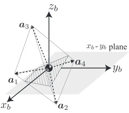
The preceding discussion shows that at least four thrusters are necessary to control the satellite’s three-dimensional attitude. Furthermore, the fourth thruster must be placed in the opposite direction to a point inside the triangular pyramid in Fig. 2.4. Then, these four thrusters give us four choices to select three thrusters and consequently formulate one large triangular pyramid containing the origin inside it as shown in Fig. 2.5. Thus, this four-thruster configuration can generate control torques to arbitrary directions in the xb-yb plane. (From a different point of view, these four thrusters can generate any directional control torque in three- dimension, and therefore this result indicates the same result derived by Sidi [38].)

13

(18)

Figure 2.3: Third thruster allocation required for controllability.

2.3 Kinematic equations of motion

There are several sets of attitude parameters to describe kinematic equations of a spacecraft. Although Euler angles, quaternion, and Rodrigues parameters are most frequently used, this chapter uses the wz-parameters proposed by Tsiotras and Longuski [45] to represent the satellite attitude. The attitude representation with wz-parameters decouple the parameter z from the parameters w₁ and w₂, and the resulting equations are further simplified by combining the parametersw1

and w2 into a complex form as w = w1+iw2, where i is an imaginary number.

The kinematic equations with wz-parameters are obtained with two successive rotations, whereas Euler angles take three rotations and quaternions and Rodrigues parameters use one rotation. In the wz-parameters, an inertial frame is rotated to coincide with the satellite-fixed frame through the following two rotations. The first rotation is defined about the zb-axis, and the second one is about an axis in thexb-yb plane and denoted byw1 andw2. The kinematic equations of the satellite can be expressed with the following two differential equations [45].

˙

w = −iωzw+ ω 2 + ω¯

2w², (2.18)

˙

z = ω_z+ i

2(¯ωw−ωw),¯ (2.19)

where angular velocities of the satellite are also written as a complex variable, i.e., ω=ωx+iωy, and ¯∗indicates its complex conjugation.

(19)

-

Figure 2.4: The control torques formulated with three thrusters.

2.4 Control Law

As seen in the dynamic and kinematic equations, the attitude parameters and the control torques are decoupled. That is, no input torques appear in the kinematic equations. Thus, we consider the angular velocities around the xb- and yb-axes in the kinematic equations as virtual inputs.

Substituting Eq. (2.18) into the relation d

dt|w|² = 2Re( ˙ww),¯ (2.20) we obtain

d

dt|w|² = (1 +|w|²)Re(ωw).¯ (2.21) Equation (2.19) corresponds to the following equation.

˙

z = Im(ωw¯+ωz). (2.22)

It should be noted that the real part of ωw¯ appears only in Eq. (2.21), whereas the imaginary part ofωw¯ is only in Eq. (2.22). Thus, we design the virtual input

15

(20)

-

Figure 2.5: The control torque formulated with four thrusters ωd as the following form:

ωd=−κw−iµz−λωz/σz

¯

w , (2.23)

where κ, µ, and λ are positive constant gains. In the controller, λωz/σz is the additional term modified from the controller shown in [46] and behaves to change the control gain depending on the moment of inertia ratio σz. That is, when the satellite has a near-axisymmetric moment of inertia, the value ofσzbecomes small, and consequently it makes the control gain large.

Using the virtual inputs, we can obtain the following equation.

d

dt|w|² = −κ(1 +|w|²)|w|², (2.24)

˙

z = −µz+ (1 +λ/σz)ωz. (2.25) The integrals of these equations are given as follows

|w|² = 1

ce^κt−1, (2.26)

z = e^−µt

* z(0) +

+

e^µt(1 +λ/σz)ωzdt ,

. (2.27)

(21)

Thus bothw- andz-parameters exponentially converge to zero at the rate specified by the control gains κ and µ. Furthermore, from the second term of the right- hand side in Eq. (2.23), the z- parameter must converge to zero faster than the w-parameter does. Thus, considering the degree of thew-parameter in Eq. (2.26), we should design the gains as µ >κ/2.

The virtual inputs are realized using actual input torques through the dynamic equations. To simplify the expression, we combine the control torques Tx and Ty

in the following complex form

T =T_x^" +iT_y^", (2.28)

where T_x^" := Tx/Jx and T_y^" :=Ty/Jy. The error of the angular velocity is defined as

e=ω−ωd. (2.29)

Then substituting Eq. (2.23) into Eq. (2.29) and differentiating it with respect to time, we obtain the following equation.

˙

e=σxωyωz+T_x^" +i(σy +ωxωz+T_y^") +κ-

−iωzw+ω 2 +ω¯

2w². +iµ

*Im(ωw¯+ωz)

¯

w − z

¯ w²

-iωzw¯+ ω¯ 2 +ω

2w¯².,

. (2.30) Thus, we design the following control law.

T =−B(ω,ωz)−κ-

−iωzw+ ω 2 +ω¯

2w².

−iC(w, z,ω,ω_z)−α /

ω+κw+iµz−λωz/σz

¯ w

0

, (2.31) where

B(ω,ω_z) = σ_xω_yω_z+iσ_yω_zω_x, (2.32)

C(w, z,ω,ωz) = µIm(ωw¯+ωz)−λωxωy

¯

w + µz−λωz/σz

¯ w²

-iωzw¯+ω¯ 2 +ω

2w¯². , (2.33) and α is a positive control gain. Consequently, the angular rate error has the following expression.

˙

e=−αe. (2.34)

This indicates that the error parameter exponentially converges to zero at the convergence rate determined by the control gain α. Thus, the control torques shown in Eq. (2.31) can implement the designed virtual inputs.

17

(22)

The thruster forces to generate the control torques shown in Eq. (2.31) can be calculated through Eq. (2.16) as

f =A^"⁺T. (2.35)

Note that the matrix A^" is not full rank for any parallel thruster configuration.

Thus the inverse matrix of A^" should be calculated using a pseudo inverse matrix

A^"⁺ to minimize the norm of f.

2.5 Numerical Simulations

This section shows some simulation results to demonstrate the validity of the derived control law. From the above discussion, we deal with a satellite that equips three thrusters oriented parallel to the satellite’szb-axis.

Since each column vector of the matrix A^" in Eq. (2.16) expresses the torques when fi = 1 (i = 1,2,3), a thruster configuration graph gives us a clue for better thruster configurations. For example, a thruster configuration whose geometric center coincides with the satellite’s mass center can equally distribute the load of the control torques to each thruster. This feature is exploited to determine the thrusters’ attachment positions in the following simulations. When the thrusters’

magnitude ranges are different, divide the distances from the mass center to the thrusters by the maximum magnitudes. Then, that result helps us to find a better thruster configuration to distribute the control torques.

Here we assume that three thrusters have the same magnitude range. Since the regular triangle configuration should be efficient for three thrusters, we firstly deal with the thruster configuration depicted in Fig. 2.6. In this configuration, all distances from the mass center to the thrusters are equal, and the geometric center of the triangle coincides with the mass center. The following matrix shows the thruster configuration.

Aa =



 0.50 −1.00 0.50 0.87 0.00 −0.87 0.00 0.00 0.00



. (2.36)

Table 2.1 summarizes the simulation parameters and the initial condition: the satellite’s moment of inertia, the angular rate, the attitude angle, and the control gains used in the simulations. The initial attitude angles are expressed with the ZYX Euler angles for better understandings. Since the inertial frame can be set arbitrarily, without loss of generality, the target state is defined as zero-attitude angles in the simulations. Note that the controller in [46] cannot be applied to the asymmetric moment of inertia case, and that Morin’s time-varying feedback controller [13] suffers from a slow convergence rate.

(23)

Table 2.1: Simulation parameters Moment of inertia Jx, Jy, Jz[kgm²]

Asymmetric case: 15.0, 10.0, 6.0 Near-axisymmetric case: 15.0,14.0,6.0 Initial angular rateωx(0),ωy(0),ωz(0)[rad/s] 1.0, 1.0, 1.0

Initial attitude angle φ(0),θ(0),ψ(0)[deg] 0.0, 45.0, 45.0 Control gains α,κ, µ,λ 10.0, 0.2, 5.0, 2.0

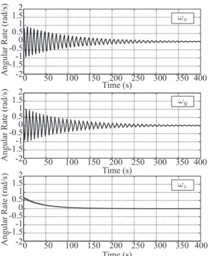
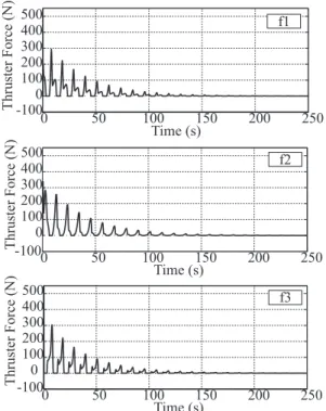
Figure 2.6: Three-thruster configurations view from the positive zb-direction The simulation results for the asymmetric moment of inertia in Table 2.1 are shown in Figs. 2.7, 2.8, and 2.9. Figures 2.7 and 2.8 indicate the time profiles of the angular velocities and the wz-parameters, respectively. Figure 2.9 is the time profile of the Euler angles and is added for better understanding of the attitude motion. For the near-axisymmetric case, the time profiles of the angular velocities, the wz-parameters, and the Euler angle expressions are shown in Figs. 2.10, 2.11, and 2.12, respectively. The convergence of the three attitude parameters to zero means that the satellite’s attitude has been controlled to the target attitude successfully. Figure 2.13 describes the time profiles of the thruster forces for the symmetric moment of inertia model, and it is shown that the required forces are kept positive or zero during the attitude maneuver. These results indicate that the proposed controller is valid and effective, because it is applicable for any satellites regardless of its moment of inertia, and because the convergence rate is not slow

19

(24)

for both moment of inertia cases.

Next, we examine the different thruster configuration depicted in Fig. 2.6b.

In this configuration, though the distances to the three thrusters are equal, the geometric center of the triangle coincides with the mass center. The configuration matrix is expressed as follows.

A_b =



 0.28 −1.00 0.28 0.96 0.0 −0.96 0.00 0.00 0.00



. (2.37)

Figure 2.14 shows the time profiles of the thruster forces for the symmetric moment of inertia case. Thus, comparing Fig. 2.13 with Fig. 2.14, it is verified that the regular triangle configuration shown in Fig. 2.6a requires lower thruster magnitudes than the ones for the thruster configuration shown in Fig. 2.6b. It indicates that proper thruster configuration can reduce the required forces.

!"#$%&'(

)*+,-./%0.1$%&/.23'()*+,-./%0.1$%&/.23'()*+,-./%0.1$%&/.23'(

6 76 866 876 966 976

:8;7:9:8 :6;76;78;7689

%

6% 76 866 876 966 976

%

Figure 2.7: The time histories of the angular velocity(asymmetric)

(25)

!"#$%&'(

wz-parameterswz-parameterswz-parameters

> ?> 8>> 8?> 9>> 9?>

<>@?

>

>@?

8

%

> ?> 8>> 8?> 9>> 9?>

<>@?

>

>@?

8

%

> ?> 8>> 8?> 9>> 9?>

<>@?

>

>@?

8

%

Figure 2.8: The time histories of the wz-parameters(asymmetric)

good bad

!"#$%&'(

Euler angles(deg)

!"#$%&'(

Euler angles(deg)

!"#$%&'(

Euler angles(deg) Euler angles(deg) Euler angles(deg) Euler angles(deg)

1 21 311 321 411 421

591571 541417191:11

%

Figure 2.9: The time histories of the ZYX Euler angles(asymmetric) 21

(26)

!"#$%&'(

)*+,-./%0.1$%&/.23'(

!"#$%&'(

)*+,-./%0.1$%&/.23'(

!"#$%&'(

)*+,-./%0.1$%&/.23'(

6 76 866 876 966 976 <66 <76 =66 :9

:8;7:8 :6;76;78;7689

:9 :8;7:8 :6;76;78;7689

%

6 76 866 876 966 976 <66 <76 =66

%

6 76 866 876 966 976 <66 <76 =66

%

Figure 2.10: The time histories of the angular velocity(near-axisymmetric)

!"#$%&'(

wz-parameters

!"#$%&'(

wz-parameters

!"#$%&'(

wz-parameters

9?>

%

> ?> 8>> 8?> 9>> 9?> :>> :?> ;>>

<8

<>@?

>

>@?

8 8@?

9

%

> ?> 8>> 8?> 9>> 9?> :>> :?> ;>>

<8

<>@?

>

>@?

8 8@?

9

%

> ?> 8>> 8?> 9>> 9?> :>> :?> ;>>

<8

<>@?

>

>@?

8 8@?

9

%

Figure 2.11: The time histories of the wz-parameters(near-axisymmetric)

(27)

good bad

!"#$%&'(

Euler angles(deg)

!"#$%&'(

Euler angles(deg)

!"#$%&'(

Euler angles(deg)

421

%

1 21 311 321 411 421 611 621 711

1 21 311 321 411 421 611 621 711 521

1 21 311 321

521 1 21 311 321

%

Figure 2.12: The time histories of the ZYX Euler angles(near-axisymmetric)

!"#$%&'(

!)*+',$*%-.*/$%&0(

!"#$%&'(

!)*+',$*%-.*/$%&0(

!"#$%&'(

!)*+',$*%-.*/$%&0(

bad good

1 21 311 321 411 421

53113114116117112111

%

1 21 311 321 411 421

5311 1 311 411 611711 211

%

1 21 311 321 411 421

5311 1 311 411611 711 211

%

% 83

84

86

Figure 2.13: The time histories of the thruster forces in Fig. 2.6(a) 23

(28)

bad good

!"#$%&'(

!)*+',$*%-.*/$%&0(

!"#$%&'(

!)*+',$*%-.*/$%&0(

!"#$%&'(

!)*+',$*%-.*/$%&0(

1 21 311 321 411 421

5311 3111 411611 711211

%

1 21 311 321 411 421

5311 1 311 411 611 711 211

%

1 21 311 321 411 421

53113114116117112111

%

% 83

84

86

Figure 2.14: The time histories of the thruster forces in Fig. 2.6(b)

(29)

2.6 Summary of Chapter 2

This chapter has discussed the minimum necessary number of thrusters required for a satellite’s three-dimensional attitude control. Considering the satellite’s nonholonomic constraint and applying the Minkowski-Farkas theorem, we have analytically shown that three thrusters placed in parallel to the satellite’s one principal axis can control the satellite attitude motion. Furthermore, a nonholonomic controller is obtained using the wz-parameters fore the attitude representation. The controller is effective for any satellite regardless of its moment of inertia. Numer- ical simulations have demonstrated the effectiveness of the proposed control law, and the efficiency of a properly placed thruster configuration has been numerically verified.

25

(30)

Chapter 3 Position and Attitude Control of an Underactuated Satellite with Constant Inputs

This chapter discusses a position and attitude control of an underactuated satellite which uses only on-offthruster mechanisms. Though several studies deal with a position and attitude control of a satellite, they assume enough number of actuators, i.e. translational forces are independent from rotational torques and vice versa.

On the other hand, this chapter assumes only four on-offthrusters are equipped on a satellite, and thus they cause a coupled motion between the translation and the rotation. The control system becomes a second-order nonholonomic system with input constraints, and the input constraints disable us to apply most of existing control theories. The purpose of this chapter is to show that a satellite’s position and attitude can be simultaneously controlled with a small number of thrusters.

First, considering the input constraints, we obtain a three-step control procedure of a satellite attitude. The control procedure is then extended to the control of the satellite’s translational and rotational motion in three-dimensions based on analytic solutions. In section 3.7, the proposed control technique is applied to a practical example of a lunar landing mission. For the lunar landing, a powered descending phase is studied considering the satellite mass change due to the fuel consumption of thrusters. In spite of the mass change of the satellite, the proposed analytical solution can accurately approximate the position and attitude of the satellite, and consequently enable the pinpoint landing. Numerical simulation results demonstrate the validity of the proposed controller for both the free-floating satellite and the lunar lander.

(31)

3.1 Equations of motion

This chapter considers the Cartesian coordinates {X,Y,Z} as an inertial reference system and denotes the principal axes of a satellite as{xb,yb,zb}. The origin of the body-fixed frame is placed to the satellite’s mass center.

3.1.1 Thruster Configuration

The minimum thruster configuration to control both position and attitude of a satellite is difficult to be determined because of the nonholonomic and input constraints. As mentioned in Chapter 1 and Chapter 2, Sidi [38] claims that the minimum number of thrusters to control a satellite’s attitude is four from a discussion on generating arbitrary control torques around three axes. The paper, however, does not consider nonholonomic constraints of the satellite’s rotational motion. The minimum number of thrusters thus has not been discussed considering the nonholonomic constraints, and a new result would be obtained. Also, some theorems to prove controllability of nonlinear systems, e.g. Sussmann [20] or Good- wine [21], are not applicable because of unilateral and constant inputs. This paper therefore deals with a thruster configuration which can generate two independent control torques around the principal axes. Although this thruster configuration has not been analytically proved to be the minimum number of thrusters because there is no control theories to discuss the controllability with constant inputs, we predict this thruster configuration enables the position and attitude control of a satellite from the viewpoint of nonholonomic attitude control shown in Chapter 2.

This chapter, for simplicity, places four thrusters to be parallel to the satellite’s principal axisyb as shown in Fig. 3.1, and assumes that all thrusters generate the same magnitude of constant force Fc and have the same length of moment arm about the xb- and zb-axes. Then, in spite of the constant and unilateral inputs, this thruster allocation can generate a pure rotational torque, i.e. without the influence about the other two axes, around the xb- and zb-axes, respectively.

The thruster combinations below are employed to control the attitude of the satellite:

T_x⁺ :f3 =f4 = Fc, f1 =f2 = 0, (3.1) T_x⁻ :f1 =f2 = Fc, f3 =f4 = 0, (3.2) T_z⁺ :f1 =f4 = Fc, f2 =f3 = 0, (3.3) T_z⁻ :f2 =f3 = Fc, f1 =f2 = 0, (3.4) where T_j⁺ and T_j⁻ (j = x, z) denote positive and negative directional control torques around the xb- and zb-axes, respectively. Note that, the thrusters cannot attenuate the translational velocity without an attitude change due to the unilateral constraint on the thrust forces. Thus, both the satellite’s translational and rotational motion must be controlled simultaneously.

27

(32)

Figure 3.1: Thruster configuration.

3.1.2 Rotational Equations of Motion

The dynamics of an underactuated spacecraft with two control torques, are written as

˙

ωx = σxωyωz +Tx/Jx, (3.5)

˙

ωy = σyωzωx, (3.6)

˙

ωz = σzωxωy +Tz/Jz, (3.7) whereωk andJk(k =x, y, z) denote an angular velocity and the principal moment of inertia, respectively, andσk(k=x, y, z) are the moment of inertia ratios defined in Eqs. (2.4), (2.5), and (2.6). Similarly to Chapter 2, but for different axes, we assume that σy "= 0, i.e. Jx "=Jz, otherwise Eq. (3.6) indicates that the rotational velocity around theyb-axis becomes uncontrollable.

Let R_bi denote a direction cosine matrix (DCM) from the inertial frame to the body-fixed frame. The relation between the DCM and the angular velocities satisfies the following equation [47].

R˙bi =Q(ω)Rbi, (3.8)

where Q(ω) expresses the skew-symmetric matrix which consists of the angular velocity vectorω, and is written as

Q(ω) =



 0 ωz −ωy

−ωz 0 ωx

ω −ω 0



. (3.9)

(33)

This chapter also represents the satellite attitude angles using thewz-parameters, and the parameters make it possible to foresee a proper control procedure and control the satellite attitude to a desired target with fewer number of maneuvers as shown in the later section.

The DCM using the wz-parameters is described as Rbi = 1

1 +w²₁ +w²₂

·



 (1 +w²₁+w₂²)c−2w₁w₂s (1 +w₁²−w₂²)s+ 2w₁w₂c −2w₂ 2w1w2c−(1−w²₁+w²2)s 2w1w2s+ (1−w₁²+w22)c 2w1

2w2c+ 2w1s 2w2s−2w1c 1−w²₁ −w²₂



, (3.10) where c := cosz and s := sinz, respectively. The kinematic equations of the satellite are again written as follows:

˙

w1 = ωzw2+ωyw1w2+ωx

2 (1 +w12−w²₂), (3.11)

˙

w2 = −ωzw1+ωxw1w2+ ωy

2 (1 +w22−w²₁), (3.12)

˙

z = ωz−ωx+ωyw1. (3.13)

3.1.3 Translational Equations of Motion

A satellite’s translational motion in an inertial frame is expressed with a DCM from the inertial frame to the body-fixed frame. Since the DCM is an orthonormal matrix, the DCM from the body-fixed frame to the inertial frame has the relationship Rib=R^T_bi. Thus, the translational equations in the Cartesian coordinate are written as

mV˙ =RibF, (3.14)

wherem,V, andF denote the mass of the satellite, a translational velocity vector in the inertial frame, and an external force vector in the body-fixed frame, respectively. Also, the kinematic equations for the translational motion are described as

X˙ =V, (3.15)

where X indicates the satellite’s position vector in the inertial reference frame.

When the thrusters are allocated parallel to the yb-axis, the components of Eq.

29

(34)

(3.14) are simplified as follows.

mV˙X = Fy

1 +w₁²+w²₂

12w1w2cosz−(1− −w²₁+w²₂) sinz2

, (3.16) mV˙Y = Fy

1 +w₁²+w²₂

12w1w2sinz+ (1−w²₁+w₂²) cosz2

, (3.17) mV˙Z = 2Fy

1 +w₁²+w²₂w1. (3.18)

3.2 Attitude Control Method

Since the thruster forces are constrained to be constant, the constraints make it difficult to design a feedback controller, and control theories for nonlinear systems are not directly applicable to the system in this chapter. This section thus shows a new attitude control method using thewz-parameters. Although quaternions or Euler angles can be used for the satellite’s attitude control, we have shown that the wz-parameters enable control of the satellite’s attitude with only three steps [48].

In the following discussion in this chapter, the satellite is assumed to have no initial angular velocity because Kojima [49] shows that two constant torques around two principal axes of a satellite can stabilize the satellite’s angular velocities to zero based on the manifolds discussed by Livneh [50].

The attitude control method proposed in this chapter consists of three steps as summarized in Table 3.1. Because the control inputs are constrained to be constant, analytic solutions for a single spin motion are derived for each maneuver and they provide proper input timings to control the attitude parameters to zero sequentially. In maneuver 1, for instance, after w2 is converged to zero, the next step controls w1 → 0 while w2 is kept invariant, i.e. ˙w2 = 0. Each maneuver in Table 3.1 is explained through the following discussion.

Table 3.1: Attitude control procedure.

Maneuvers Target state Input timing

1 (w1,0, z) w1,z:arbitrary φd = _2J^T^z⁻_z(∆t⁻)²+ω⁻_z0∆t⁻ 2 (0,0, z)z:arbitrary w1d= tan-

−_4J^T^x⁻_x(∆t⁻)²−^ω^x0₂⁻∆t⁻. 3 (0,0,0) zd=−_2J^T^z⁻_z(∆t⁻)²−ω⁻_z0∆t⁻

In maneuver 1, a positive control torque about the zb-axis is applied during a finite time∆t⁺to generate a single spin motion, where the superscript “+” denotes a parameter when a positive directional torque is applied. Since the single spin motion avoids the coupling effect of the angular velocity, the dynamic equations