Theoretical Study on
Thermodynamic Properties of Ice and Clathrate Hydrate
September, 2020
•
Muhammad Mahfuzh Huda
The Graduate School of Natural Science and Technology
(Doctor Course)
Okayama University
Table Of Content
Table Of Content ...1
Chapter 1 ...3
Introduction ...3
1.1 Water: The Molecule That Shape Our Reality ... 3
1.2 Molecular Simulations ... 5
1.3 Hydrogen Bond ... 6
1.4 Models of Water ... 8
1.4.1 TIP4P and TIP4P/Ice Models of Water ...9
1.4.2 mW Model of Water ... 11
1.5 Negative Thermal Expansivity of Water ... 13
1.6 Clathrate Hydrate ... 14
1.7 Research Aims ... 16
1.8 References ... 17
Chapter 2 ... 22
Negative Thermal Expansivity of Ice: Comparison of the Monatomic mW Model with the All-Atom TIP4P/2005 Water Model ... 22
2.1 Introduction ... 22
2.2 Method ... 25
2.2.1 Force Field Models and Structure of Ice ... 25
2.2.2 Quasi-Harmonic Approximation ... 27
2.3 Results ... 28
2.4 Discussion ... 33
2.5 Conclussions... 41
2.6 References ... 42
Chapter 3 ... 45
On the Study of Solubility of Gas Molecules in Clathrate Hydrate ... 45
3.1 Introduction ... 45
3.2 Computational Method ... 49
3.2.1 Revised vdWP Theory ... 49
3.2.2 Thermodynamic Integration ... 52
3.2.3 Procedure For MD Simulation... 53
3.2.4 Potential Interactions... 54
3.3 Result and Discussion ... 54
3.3.1 Dissociation Pressure... 54
3.3.2 Chemical Potential of Guest Molecule Inside Clathrate Hydrate ... 57
3.3.3 The Solubility of Guest Molecule in Water with the Presence of Clathrate Hydrate 59 3.4 Conclusions ... 63
3.5 Reference ... 64
Chapter 4 ... 69
General Conclusion ... 69
Chapter 1
Introduction
1.1 Water: The Molecule That Shape Our Reality
Water is one of the most studied liquids on the earth. The importance of water is not only in the development of the earth’s atmosphere but also the formation of the solar system. The most compelling theory of the beginning of the universe reveals that as soon as the oxygen is formed, it reacts with hydrogen forming water[1]. Two of the most reactive elements that present at the beginning of the universe react to produce a single unique molecule that still amazes us until today. Clouds in the skies, a crust of icebergs in the arctic and the vast ocean that form the geological landmarks of our earth, all consist of this tetrahedral molecule called water.
Water plays an important role in the field of chemistry, biology and geology.
A satisfactory explanation for the behaviour of water under various conditions is necessary for a certain field of sciences. For instance, climate science needs information on the behaviour of nanodroplet of water to understand the cloud formations[2], biophysics refer to the cohesion properties of water in a small slit to explain the transport mechanism of water from the root to the tip of the leaves[3–5], and planetary science investigates the ice formation on different thermodynamics conditions to understand the planetary surfaces[6]. Some notable physical properties are manifested by water such as: the maximum density in the liquid form (at 4°C), the Mpemba effect that hot water may freeze faster than cold water, diverse crystalline polymorphs (more than 18 ices and still counting), the large heat capacity for a very simple and lightweight molecule, the high-motilities of proton and hydroxide ions under an electric field[7,8]. Those have shaped the physical reality we experience in
daily life. If water does not display such anomalies, there is no chance that life will emerge on the earth.
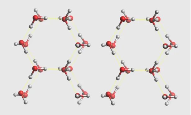
Ordinary ice, known as hexagonal ice (Ice Ih) has a crystal arrangement where each water molecule forms hydrogen bonds to 4 nearest neighbours[9]. A water molecule acts as a hydrogen donor to two of its neighbours and the lone pairs of electrons from oxygen accept hydrogens from the remaining two. These hydrogen bonds are geometrically arranged with local tetrahedral symmetry. However, the bond angle of the water molecule (104.5) is slightly less than the tetrahedral angle (109.5 )[7]. A similar arrangement is also found in clathrate hydrate, except there are possibilities of forming pentagonal rings.
Figure 1: The spacial arrangement of the common ice crystal (Ice Ih), yellow dotted line is the hydrogen bonds.
Scientists still exploring the behaviour of one of the most abundant liquid on the earth surface. Thus, it is essential to study liquid water and crystalline ices from microscopic perspectives with the intermolecular interactions to describe the hydrogen bonds accurately. In this study, we will focus our attention on the thermodynamic properties of ice and clathrate hydrate, whose main component is water.
1.2 Molecular Simulations
Due to the rapid development of computer hardware and software, computer simulation becomes more popular and accessible to chemists. Molecular simulation provides a possibility to describe the relation between microscopic details of a system and the macroscopic properties measurable from experiments. Thus, molecular simulation becomes a new powerful tool in studying the thermodynamic properties of water. Another advantage using molecular simulation is the flexibility in manipulating the thermodynamic conditions as well as extracting quasi-experimental data allow us to acquire specific information that is not readily measurable from experiments[10].
Monte Carlo (MC) and molecular dynamics (MD) simulations are the most commonly used techniques in molecular simulation. The basic idea of MC simulation is to generate representative configurations under specific thermodynamic conditions [11,12]. To accurately represent real systems, configurations generated in MC simulations should be averaged over a large number of the generated configurations.
The probability of one configuration is determined from a relevant thermodynamic property. A sequence of the configurations are generated via the Markov chain. Thus, ordinary MC simulations cannot provide time-dependent properties and are used to study the thermodynamics of a real system. To access information of the time evolution of the system, we use MD simulation. In MD simulations, we calculate the forces from the intermolecular interactions to solve the equation of motion to investigate the microscopic structure as well as the macroscopic properties comparable to the experimentation. The popularity of MD simulations is due to the ability to study a time-dependent phenomenon such as ice nucleation inside nanotube pores[13], the formation and dissociation of clathrate hydrates[14,15] and even to predict the structure of a protein in biological systems[16]. In theoretical chemistry studies both MC and MD simulations are often used simultaneously to gain the advantage of both methods[11,12].
However, a number of difficulties are still present in application of both MC and MD: 1) demanding of heavy computational power for simulation of large systems,
2) limitations on the accuracy of the computational model to mimic the real system, and 3) limitation of the computational techniques effectively investigates the nucleation process[17,18].Some techniques have been developed to overcome such problems, for instance, the periodic boundary condition(PBC) applied in order to describe the macroscopic system with a limited number of molecules [19], the anisotropic united atom (AUA) and coarse-grained molecular model used to simplify the molecular interactions without losing the accuracy[20]. Simpler pair interaction models and overall calculation technique with a prominent accuracy is still demanding[17].
1.3 Hydrogen Bond
The molecular structure of water has long been described by chemists. In the geometrical perspective, the nuclei of oxygen and two hydrogen atoms form an isosceles triangle with the O-H covalent bond of length 0.9572 Å and the H-O-H angle of 104.52 [21,22]. This specific information is important to develop the water model in the molecular simulation study. In the request to explain the properties of water, one might encounter the concept of the “hydrogen bond,” which was first introduced by Latimer and Rodebush[23]. This is based on the specific interaction that occurs between hydrogen and electronegative atoms such as nitrogen, oxygen, fluorine and chlorine. In the case of water, hydrogen bonds arise from a fairly strong electrostatic interaction between a positively charged hydrogen on one water molecule and a negatively charged site on another water molecule.
Two water molecules could form a hydrogen bond when the distance between the nucleus of oxygen atoms in a pair of water molecules the (O—O) is 3.10 Å and the O—H--O angle is 146 °. When a pair of water molecules have a distance greater than 3.10 Å or the O—H--O angle is less than 146 °, the hydrogen bond can be considered to be broken[24,25].
The presence of hydrogen bonds in water induces a three-dimensional tetrahedral network structure affecting the properties of water in gas, liquid, and solid
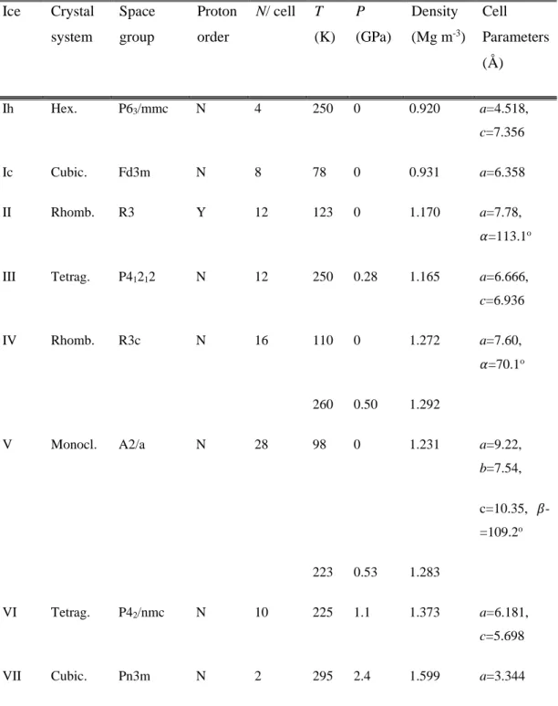
forms. In the solid forms the hydrogen bonds combined with the lone pair electrons of oxygen allow water molecules to form ice polymorphs. Some properties of those polymorphs are tabulated in Table. 1.
Table 1: Structures of the crystalline of water.
Ice Crystal system
Space group
Proton order
N/ cell T (K)
P (GPa)
Density (Mg m-3)
Cell Parameters (Å)
Ih Hex. P63/mmc N 4 250 0 0.920 a=4.518,
c=7.356
Ic Cubic. Fd3m N 8 78 0 0.931 a=6.358
II Rhomb. R3 Y 12 123 0 1.170 a=7.78,
𝛼=113.1o
III Tetrag. P41212 N 12 250 0.28 1.165 a=6.666, c=6.936
IV Rhomb. R3c N 16 110 0 1.272 a=7.60,
𝛼=70.1o
260 0.50 1.292
V Monocl. A2/a N 28 98 0 1.231 a=9.22,
b=7.54, c=10.35, 𝛽-
=109.2o 223 0.53 1.283
VI Tetrag. P42/nmc N 10 225 1.1 1.373 a=6.181,
c=5.698
VII Cubic. Pn3m N 2 295 2.4 1.599 a=3.344
VIII Tetrag. I41/amd Y 8 10 2.4 1.628 a=4.656, c=6.775
IX Tetrag. P41212 Y 12 165 0.28 1.194 a=6.692,
c=6.715
X Cubic. Pn3m n/a 2 300 62 2.79 a=2.78
XI Ortho. Cmc21 Y 8 5 0 0.934 a=4.465,
b=7.858 c=7.292
XII Tetrag. I42d N 12 260 0.50 1.292 a=8.304,
c=4.024
*Taken from Petrenko F. V. and Whitworth W. R (1999)4
1.4 Models of Water
The discovery of various anomalous properties of water from the experimental investigations leads to comprehensive understanding of water. Those discoveries also encourage theoretical scientists to propose a better model of water. Since the implementation of computational chemistry, idea to build a better model of water molecule arises from different perspectives. This results in more than a hundred water- models. However, it is only a few that can describe behaviours of the anomalous properties of water with a high accuracy.
In most cases of simulation of simple liquids, one might reproduce physical properties of the compound that are in agreement with the experiment using a good and reliable pair potential. However, in the case of water, even if a pair potential could reproduce one aspect of water, its capability to reproduce other anomalous properties of water is still questionable. Therefore, it cannot be considered as a good and reliable model. The properties of water are determined by not only the simple dispersion force
as in the pair interaction for simple liquids but also the hydrogen-bonding, which can be described more accurately by introducing the higher-body interactions.
The development of water-water pair potential has been made since Rowlinson (1949,1951), Bjerrum (1951), Watts (1968), and many others, but none of them could reproduce the tetrahedral structure of water. In 1972 Ben-Naim and Stillinger developed a model of water based on the Bjerrum model. It finally could reproduce the roughly tetrahedrally packed geometry of water molecules. This finding initiated a new era for the development of 3-D water models. Since then, various models for 3-D water-like particles are developed and effort has been devoted to improving water interaction potentials[22].
The pair potential is not very useful in the simulation of water, so we should use the pair-effective potential. This potential consists of three terms:
(i) The strong repulsive interaction in a very close range.
(ii) The long-range electrostatic interaction.
(iii) The hydrogen bond interaction between water with its four neighbors[22,25].
An improvement of the water model is still one of the main concerns in the study of water and might possibly be a never-ending process. Some of the most notable water models are Mercedes-Benz[22], SPC[27], SPC/E[28], TIP3P[29], TIP4P[29]
and TIP4P/Ice[29].
1.4.1 TIP4P and TIP4P/Ice Models of Water
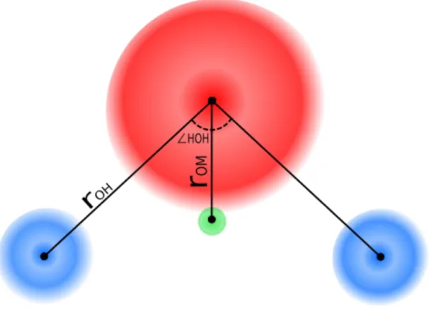
TIP4P potential is known as the most popular model because of its ability to reproduce several anomalous properties of water. The model has been used for more than decades and is still commonly used in molecular simulations or as a reference in comparison with the new model. This model consists of four interaction sites, each represented by a green sphere for a negative charge site, two blue ones for positively
charged hydrogens, and a red one for Lennard Jones interaction sitting on the oxygen atom as shown in Figure 2:
Figure 2: TIP4P Model of Water
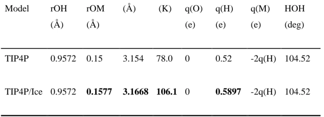
The TIP4P potential recovers the various properties of liquid water better than the other models at the time of its proposal. The model, however, is not sufficient to reproduce each density of ice polymorphs and phase diagram of water with great accuracy. To settle this problem, a similar model called TIP4P/Ice has been developed by Abascal et al. in 2005. Table 2 shows the parameters of the model; bold fonts display the distinct parameters for the TIP4P and the TIP4P/Ice model. The new model is able to reproduce the density data of several water polymorphs with better accuracy than other models[30].
Table 2: Parameters of the water models
Model rOH
(Å)
rOM (Å)
(Å) (K) q(O) (e)
q(H) (e)
q(M) (e)
HOH (deg)
TIP4P 0.9572 0.15 3.154 78.0 0 0.52 -2q(H) 104.52
TIP4P/Ice 0.9572 0.1577 3.1668 106.1 0 0.5897 -2q(H) 104.52
*Taken from Abascal et al. (2005)[29]
Because both models have four interaction sites, they are computationally expensive. This gives rise to a challenge to invent a coarse-grained model[31].
1.4.2 mW Model of Water
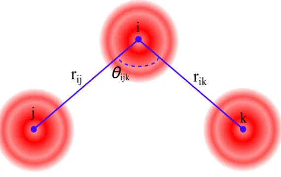
A simple water model has been proposed by Molinero in 2009, which is based on the Stillinger-Weber (SW) silicon model[32]. This model is simpler than the TIP4P since it has only one interaction site. Besides the ability in reproducing various properties of water and ice with high accuracy, the model also favourable in computational cost[18]. Illustration of the model shown as:
Figure 3: The mW model of water for three molecules of water. Each molecule of water consists of only one interaction site.
The origin of mW model is adopted from the SW-silicon model by changing several parameters. Molecular formation of water is similar to silicon giving the possibility to modify SW-silicon model to a model for water (mW). Besides water and silicon, the model could be used for simulation of germanium or carbon, since those atoms have tetrahedral coordination in low pressure regime.
mW model demands less computational cost than the TIP4P, TIP4P/Ice and SPC/E model. Compared to the SPC/E model, the least expensive atomistic model, mW model is 180 times faster. A considerable difference in speed arises from the smaller number of particles involved in the calculation (1 versus 3), the longer time step (10 versus 1.5fs) for integration of equations of motion and shorter interaction range (cutoff at 4.32 Å versus Ewald sums). Less computational cost in computation is very valuable because we can treat a longer time or larger system in simulation.
1.5 Negative Thermal Expansivity of Water
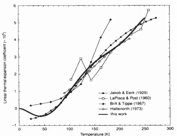
One unique property of ice is the observation that the volume shrinks upon heating at temperature below 63 K. This phenomenon has been discovered more than three decades ago and found only in tetrahedral-structured crystals at a very low temperature. The negative thermal expansivity of ice at very low temperature has been observed in experiments. The most notable experimental data are disclosed by Röttger et al. in 1994 and updated in 2012 using the synchrotron X-ray measurement method that gave better result than previous investigation as seen in Figure 4 [33].
In 1997, Tanaka investigated the origin of the negative thermal expansion using a simple water model. He employed the TIP4P potential model of water and calculated the free energy utilizing the quasi-harmonic approximation [34]. Result of the study shows a good agreement with the experimental observations. This characteristic of crystal seems common to the four-coordinated molecules.
However, the negative thermal expansion is not only observed in water, but some other crystals with open structures also share the same property. Silicon, quartz and zeolites exhibit the negative thermal expansion. Thus, with the development of mW water model from the original SW-silicon model, we attempt to reproduce the negative thermal expansion of ice utilizing mW water model. In chapter II, we investigate the origin of the negative thermal expansivity of ice using a monatomic water (mW) model.
1.6 Clathrate Hydrate
Gas hydrate is a crystal lattice compound built from guest molecules trapped in the cages of water molecules known as the host. The guest molecules are low-molecular- weight gas such as methane, ethane, hydrogen, CO2, propane and isobutane. The cage
Figure 4: Comparison of some literature data on the thermal expansivity coefficient for H2O ice Ih *taken from Röttger K et al. 1994.
of water in clathrate hydrate is similar to the ice structure which is formed from the tetrahedrally coordinated hydrogen bonds. The guest molecules trapped inside the cage do not have any chemical bond with the water molecules constituting cage or with any gas molecules outside the cage[35,36].
A unique property of gas hydrate is the ability to keep a large amount of gas in its crystal structure. For example, 1 m3of methane hydrate crystal could store 160 m3 volume of methane gas at 273 K and 0.1 MPa. A significant amount of methane hydrate crystals is found in the ocean floor and permafrost. The fact that gas hydrates could store abundant amounts of greenhouse gases such as (methane, carbon dioxide, etc.) means that the dissociation of hydrate will speed up global warming. But the fact that clathrate hydrate can contain a large amount of gases reveals that it is not only the source of gas but also a potential gas storage[37,38]. Gas hydrates naturally occur in marine environments, deep sea sediment and permafrost layers. One notable presence of the methane hydrate is in the oil industry which is blocking the pipeline causing problems for engineers[37,39].
There is an increasing interest in the study of formation and dissociation of clathrate hydrate. However, the formation and deformation of methane hydrate remain mysterious. This is due to the lack of reliable experimental methods that can provide the in-situ dynamics information on the molecular level. The condition of the system before the guest molecule is absorbed inside the cage forming hydrate crystal and before the hydrate crystal dissolves to liquid is very important information to understand the kinetics of methane hydrates [39,40].
Clathrate hydrate is a non-stoichiometric compound, a cage of clathrate hydrate can be encaged by more than one guest molecule as well as can be empty, thus the gas- water ratio in the clathrate hydrate is varied depending on the temperature and pressure of the system. Measuring the composition of clathrate hydrate with high accuracy is still a challenging issue in the field of experimental chemistry[35]. In 1965, a series of crystallographic measurements were performed to uncover the structure and composition of clathrate hydrate [35]. Based on the structural geometry, it is mainly separated into three categories: structure I (sI), structure II (sII) and hexagonal
structure (sH). By knowing the structure of clathrate hydrate, a thermodynamics model of the clathrate hydrate could be predicted using statistical thermodynamics. Since then, many approaches have been proposed to describe the thermodynamic details of the hydrate systems. In chapter III, the thermodynamic stability of clathrate hydrates are investigated for several guest species under various conditions. Special attention is focused on the water/hydrate boundary in the presence and absence of the intervening hydrate phase, where the temperature dependence of the solubility of guest species in the aqueous phase is examined.
1.7 Research Aims
Water has been the subject of many researchers not only for its role as universal solvent but also for its unique properties. The development of computational chemistry offers a new insight into exploring the behaviours of water. Understanding of the thermodynamic behavior under a specific condition is necessary for various fields of study. In this PhD thesis, I report the thermodynamic properties of ice and clathrate hydrates from theoretical calculations. Both are crystalline solids made of water molecules alone or water and small apolar molecules. Here, attention is placed on anomalous thermodynamics properties caused by water molecules.
In this study, first we focus on testing a new model of water and questioning its ability to reproduce anomalous properties of ice polymorphs. A simple prescription is proposed to recover the negative thermal expansion by re-adjusting the parameter of mW water model. We also investigate the relation between thermal expansion, Grüneisen parameter, and the vibrational free energy in the mW model and compare it with an all-atom water model such as TIP4P/Ice.
The second is associated with the temperature dependence of the solubility of apolar molecules in water in the presence or absence of the clathrate hydrates containing the apolar molecules. The formation of clathrate hydrate in the pipeline gives trouble to the transport of oil and gas. The fact that the formation of the clathrate hydrate are mainly affected by the solubility of natural gases in solution phase inspires
us to explore more. We rise a question about the solubility of various gases in clathrate hydrate and in the solution phase. By obtaining this information we explore the mechanism underlying the formation and deformation of gas hydrate.
1.8 References
1. Ball P. H2O. A Biography of Water. Orion Books Ltd, London; 2000.
2. Malek SMA, Poole PH, Saika-Voivod I. Thermodynamic and structural anomalies of water nanodroplets. Nat Commun. 2018;9: 2402.
doi:10.1038/s41467-018-04816-2
3. Steudle E. The Cohesion-Tension Mechanism and The Acquisition of Water by Plant Roots. Annu Rev Plant Physiol Plant Mol Biol. 2001;52: 847–875.
doi:10.1146/annurev.arplant.52.1.847
4. Steudle E. Transport of Water in Plants. Environment Control in Biology.
2002. pp. 29–37. doi:10.2525/ecb1963.40.29
5. Sansom MS, Biggin PC. Water at the nanoscale. Nature. 2001. pp. 156–159.
doi:10.1038/35102651
6. Baragiola RA. Water ice on outer solar system surfaces: Basic properties and radiation effects. Planet Space Sci. 2003;51: 953–961.
doi:10.1016/j.pss.2003.05.007
7. Stillinger FH. Water revisited. Science. 1980;209: 451–457.
doi:10.1126/science.209.4455.451
8. Chaplin M. Anomalous properties of water. Water structure and science [cit 2015-4-15], Web: http://www1.lsbu.ac.uk/water/water_anomalies.html 9. Petrenko VF, Whitworth RW. Physics of Ice. OUP Oxford; 1999.
10. Hansen J-P, McDonald IR. Theory of Simple Liquids. Elsevier; 1990.
11. Paquet E, Viktor HL. Molecular dynamics, monte carlo simulations, and langevin dynamics: a computational review. Biomed Res Int. 2015;2015:
183918. doi:10.1155/2015/183918
12. Gilabert JF, Gracia Carmona O, Hogner A, Guallar V. Combining Monte Carlo and molecular dynamics simulations for enhanced binding free energy estimation through Markov State Models. J Chem Inf Model. 2020.
doi:10.1021/acs.jcim.0c00406
13. Koga K, Gao GT, Tanaka H, Zeng XC. Formation of ordered ice nanotubes inside carbon nanotubes. Nature. 2001;412: 802–805. doi:10.1038/35090532 14. Yagasaki T, Matsumoto M, Tanaka H. Formation of Clathrate Hydrates of
Water-Soluble Guest Molecules. J Phys Chem C. 2016;120: 21512–21521.
doi:10.1021/acs.jpcc.6b06498
15. English NJ, Johnson JK, Taylor CE. Molecular-dynamics simulations of methane hydrate dissociation. The Journal of Chemical Physics. 2005. p.
244503. doi:10.1063/1.2138697
16. Karplus M, Petsko GA. Molecular dynamics simulations in biology. Nature.
1990;347: 631–639. doi:10.1038/347631a0
17. Sosso GC, Chen J, Cox SJ, Fitzner M, Pedevilla P, Zen A, et al. Crystal Nucleation in Liquids: Open Questions and Future Challenges in Molecular Dynamics Simulations. Chem Rev. 2016;116: 7078–7116.
doi:10.1021/acs.chemrev.5b00744
18. Molinero V, Moore EB. Water Modeled As an Intermediate Element between Carbon and Silicon†. The Journal of Physical Chemistry B. 2009. pp. 4008–
4016. doi:10.1021/jp805227c
19. Allen MP, Tildesley DJ. Computer Simulation of Liquids. Oxford Scholarship Online. 2017. doi:10.1093/oso/9780198803195.001.0001 20. Huda M, Ulfa SM, Hakim L. Chemical Potential of Benzene Fluid from
Monte Carlo Simulation with Anisotropic United Atom Model. The Journal of Pure and Applied Chemistry Research. 2013. pp. 115–121.
doi:10.21776/ub.jpacr.2013.002.03.163
21. Császár AG, Czakó G, Furtenbacher T, Tennyson J, Szalay V, Shirin SV, et al. On equilibrium structures of the water molecule. J Chem Phys. 2005;122:
214305. doi:10.1063/1.1924506
22. Ben-Naim A. Molecular Theory of Water and Aqueous Solutions. Molecular Theory of Water and Aqueous Solutions. 2009. doi:10.1142/7136
23. Latimer WM, Rodebush WH (1920) Polarity and ionization from the standpoint of the Lewis theory of valence. J Am Chem Soc 42:1419–1433.
doi:10.1021/ja01452a015
24. Matsumoto M. Relevance of hydrogen bond definitions in liquid water. J Chem Phys. 2007;126: 054503. doi:10.1063/1.2431168
25. Maréchal Y. The H2O Molecule in Liquid Water. The Hydrogen Bond and the Water Molecule. 2007. pp. 215–248. doi:10.1016/b978-044451957- 3.50010-x
26. Eisenberg D, Kauzmann W. The Structure and Properties of Water. 2005.
doi:10.1093/acprof:oso/9780198570264.001.0001
27. Berendsen HJC, Postma JPM, Van Gunsteren WF, Hermans a. J.
Intermolecular forces. Reidel, Dordrecht Jerusalem, Israel; 1981.
28. Berendsen HJC, Grigera JR, Straatsma TP. The missing term in effective pair potentials. J Phys Chem. 1987;91: 6269–6271. doi:10.1021/j100308a038
29. Jorgensen WL, Chandrasekhar J, Madura JD, Impey RW, Klein ML.
Comparison of simple potential functions for simulating liquid water. The Journal of Chemical Physics. 1983. pp. 926–935. doi:10.1063/1.445869 30. Abascal JLF, Sanz E, García Fernández R, Vega C. A potential model for the
study of ices and amorphous water: TIP4P/Ice. J Chem Phys. 2005;122:
234511. doi:10.1063/1.1931662
31. Lu J, Qiu Y, Baron R, Molinero V. Coarse-Graining of TIP4P/2005, TIP4P- Ew, SPC/E, and TIP3P to Monatomic Anisotropic Water Models Using Relative Entropy Minimization. J Chem Theory Comput. 2014;10: 4104–
4120. doi:10.1021/ct500487h
32. Stillinger FH, Weber TA. Computer simulation of local order in condensed phases of silicon. Phys Rev B Condens Matter. 1985;31: 5262–5271.
doi:10.1103/physrevb.31.5262
33. Röttger, K.; Endriss, A.; Ihringer, J.; Doyle, S.; Kuhs, W.F. Lattice constants and thermal expansion of H2O and D2O ice Ih between 10 and 265 K.
Addendum. Acta Crystallogr. B 2012, 68, 91.
34. Tanaka, H. Thermodynamic stability and negative thermal expansion of hexagonal and cubic ices. J. Chem. Phys. 1998, 108, 4887–4893.
35. Dendy Sloan E Jr, Koh CA, Koh C. Clathrate Hydrates of Natural Gases.
CRC Press; 2007.
36. Chernov AA, Pil’nik AA, Elistratov DS, Mezentsev IV, Meleshkin AV, Bartashevich MV, et al. New hydrate formation methods in a liquid-gas medium. Scientific Reports. 2017. doi:10.1038/srep40809
37. Pellenbarg RE, Max MD. Gas Hydrates: From Laboratory Curiosity to Potential Global Powerhouse. Journal of Chemical Education. 2001. p. 896.
doi:10.1021/ed078p896
38. Kozhevnykov A, Khomenko V, Liu BC, Kamyshatskyi O, Pashchenko O.
The History of Gas Hydrates Studies: From Laboratory Curiosity to a New Fuel Alternative. Key Engineering Materials. 2020. pp. 49–64.
doi:10.4028/www.scientific.net/kem.844.49
39. Cox SJ, Taylor DJF, Youngs TGA, Soper AK, Totton TS, Chapman RG, et al. Formation of Methane Hydrate in the Presence of Natural and Synthetic Nanoparticles. J Am Chem Soc. 2018;140: 3277–3284.
doi:10.1021/jacs.7b12050
40. Gao S, House W, Chapman WG. NMR/MRI study of clathrate hydrate mechanisms. J Phys Chem B. 2005;109: 19090–19093.
doi:10.1021/jp052071w
Chapter 2
Negative Thermal Expansivity of Ice:
Comparison of the Monatomic mW Model with the All-Atom TIP4P/2005 Water Model
2.1 Introduction
Water is a most common liquid on earth, liquid water freezes into ice I under ambient pressure. One of interesting characteristics of ice I is its negative thermal expansivity at low temperatures [1–5]. This was also recovered by theoretical study [6]. The thermal expansivity of a crystal can be related to the so-called Grüneisen parameter. For a mode with frequency ν, this parameter is defined as γ = −(d ln ν/d ln V) [7]. The quantity is positive for stretching modes. This is evident from the sharp increase in the potential energy with a decrease in the bond length caused by the Pauli exclusion principle. By contrast, the Grüneisen parameter can be negative for bending modes. The negative thermal expansivity is realized when the Grüneisen parameter of the bending modes is negative and the positive contribution from the stretching modes is small enough.
The Gibbs energy calculation with the quasi-harmonic approximation is a useful computational approach to examine the thermal properties of crystals [8]. This method allows for the calculation of the temperature dependence of the equilibrium volume of a crystal, from which one can obtain the thermal expansivity. It also enables one to calculate the components of the thermal expansivity, that is, the heat capacity and the Grüneisen parameters of individual intermolecular vibrational modes. The quality of the results depends strongly on the employed force field. Excellent results can be obtained from ab initio methods considering a high level electron correlation with a large basis set, but such calculations are quite time-consuming and may
therefore not be suitable for the treatment of ice I, for which the system size and the number of examined configurations should be large enough to take the hydrogen- disorder into account [9]. In addition, properties of molecular solids, including ice, are sensitive to van der Waals interactions while empirical models to correct the van der Waals interactions for density functional theory (DFT) methods are not specialized for ice [10]. At this point, classical force fields modelled to reproduce properties of ice I work better than ab initio force fields, except for the cleavage of chemical bonds. Of course, the ab initio calculation and the path integral method are useful for examining the isotope effects and taking into account the anharmonic contributions [11–13].
Some discussions on the most effective method among these types of calculations has been conducted [14].
Here, we take advantage of the excellent reproducibility of classical force fields parameterized for liquid water and ice polymorphs. In passing, this kind of approach costs rather little, so that we can handle not only a larger number of molecules (say 1000) in the simulation cell but also many hydrogen-disordered structures, such as 100 different structures. The TIP4P/2005 model is one such classical force field [15]. A water molecule consists of one oxygen atom without charge, two positively charged hydrogen atoms, and one negatively charged site without mass. The oxygen atom interacts with oxygen atoms of other molecules via the Lennard-Jones (LJ) potential.
This model reproduces the phase diagram of ice for a wide range of pressure except for the very high pressure region [16–19]. TIP4P/2005 is a re-parameterized TIP4P model [20]. It has been demonstrated that the thermal expansivity of ice I is negative at temperatures that are under 60 K when the original TIP4P model is employed [6].
A similar method was applied to ice II and III [21].
The monatomic water (mW) model is a different type of empirical model for water [22]. This is a single site water model, and the intermolecular interactions are described by the sum of the short-ranged pair and three-body interactions. The computational cost of the mW model is quite low because the number of interaction sites is reduced and because the long-range interactions are omitted. Nevertheless, this model reproduces various properties of ice I well, such as the melting point. It has been
used frequently in molecular dynamics (MD) studies of nucleation and growth of not only ice I but also clathrate hydrates [23,24]. The mW model was developed on the basis of the Stillinger-Weber silicon model [25]. Although crystalline Si exhibits negative thermal expansivity, the Stillinger-Weber Si potential does not reproduce this anomaly [26].
The negative thermal expansivity of ice Ih has recently been measured in a and c lattice directions. Both measurements show an anisotropy in the thermal expansion between the a-axis and c-axis [3–5]. The temperature of the minimum thermal expansivity in those experiments shifts toward a low temperature, around 30 K. The negative thermal expansivity is observed for some crystals with open network structures, such as silicon, quartz, and silica zeolites. This fact suggests that the preference of a molecule for a regular tetrahedral arrangement, which is the origin of the low density of ice, is an important factor for the negative thermal expansivity [27].
In the mW model, the preference is implemented by a parameter in the three body interaction term. In this study, we calculate the thermal expansivity of ice I using the quasi-harmonic approximation and examine the effect of this tetrahedrality parameter on the thermal expansivity. We also calculate the thermal expansivity for the TIP4P/2005 model. The vibrational modes can be classified into the translation- dominant and rotation-dominant modes because it is an all-atom model. We demonstrate that the coupling between the two types of modes plays a vital role for the negative thermal expansivity of ice.
Our aim in this work is to explore how the mW model works in low temperatures by examining the thermal expansivity of ice. The original potential for the Si atom has been made, and the negative thermal expansion is recovered for amorphous Si only [28]. Therefore, it is of interest to examine if the mW model can reproduce the negative thermal expansivity and how to revise it to lead to its better reproducibility.
2.2 Method
2.2.1 Force Field Models and Structure of Ice
The potential energy of the mW model is the sum of the pairwise and three- body interactions [22]:
𝐸 = 𝜀 ∑ ∑ 𝜙2(𝑟𝑖𝑗
j>i i
) + ∑ ∑ ∑ 𝜙3(
k>j j≠i i
𝑟𝑖𝑗, 𝑟𝑖𝑘, 𝜃𝑖𝑗𝑘), (1)
with
𝜙2(𝑟) = 𝐴 [𝐵 (𝜎 𝑟)
4
− 1] exp ( 𝜎
𝑟 − 𝑎𝜎), (2)
and
𝜙3(𝑟, 𝑠, 𝜃) = 𝜆[cos 𝜃 − cos 𝜃0]2exp ( 𝛾𝜎
𝑟 − 𝑎𝜎) exp ( 𝛾𝜎
𝑠 − 𝑎𝜎). (3) The parameters are given in Table 1. The interaction is short-ranged: a molecule interacts with a different molecule only when the distance between them is shorter than aσ = 0.43065 nm. The three-body term is zero when the O-O-O angle is the tetrahedral angle of θ0 = 109.47°, and otherwise it is positive. Therefore, the preference for tetrahedral arrangements increases with the increase of the coefficient of the three body term, λ. In the mW model, this tetrahedrality parameter is set to 23.15 to reproduce various properties of ice I and liquid water [22,24,29].
Table 1. Parameters of the mW model [22].
A 7.049556277
B 0.6022245584
γ 1.2
a 1.8
λ 23.15
θ0 109.47°
σ 0.23925 nm
ε 25.895 kJ mol−1
The TIP4P/2005 model is an all-atom rigid model for water [15]. The intermolecular interactions are described by pairwise additive Coulomb and LJ interactions. A negatively charged site without mass, M, is located on the bisector of the H-O-H angle with an O-M distance of 0.01546 nm. The O-H distance and the H- O-H angle are 0.09572 nm and 104.52°, respectively. The partial charge on each hydrogen atom is 0.5564 e. The LJ parameters of the oxygen atom are 𝜎𝑂= 0.31589 nm and ε𝑂= 0.774912 kJ mol−1.
The structure of ice in this study is ice Ic, consisting of 1000 water molecules.
A hundred hydrogen-disordered ice structures without net polarization are generated for the TIP4P/2005 model by the GenIce tool [30]. For ices with the mW model, oxygen atoms are simply placed on the corresponding lattice sites. The calculations are performed for numerous densities. The shape of the cell is kept cubic throughout the expansion or compression. Periodic boundary conditions are applied to ensure that the molecules are in the bulk phase without any surface effect.
2.2.2 Quasi-Harmonic Approximation
The Helmholtz energy of ice can be expressed as:
𝐴(𝑇, 𝑉) = 𝑈𝑞(𝑉) + 𝐹(𝑇, 𝑉) − 𝑇𝑆𝑐, (4) where 𝑈𝑞(𝑉) is the potential energy at 0 K, 𝐹(𝑇, 𝑉) is the vibrational free energy, and 𝑆𝑐 is the configurational entropy. The vibrational free energy consists of the harmonic and anharmonic contributions. The anharmonic part can be ignored at low temperatures at which the potential energy surface is regarded to be parabolic in any direction. The harmonic vibrational free energy is given by:
𝐹h(𝑇, 𝑉) = 𝑘B𝑇 ∑ ln [2 sinh ( ℎ 𝜈𝑖 2 𝑘B𝑇)]
𝑖
, (5)
where ℎ is the Planck constant, 𝑘B is the Boltzmann constant, and 𝜈𝑖 is the frequency of the 𝑖-th normal mode.
The steepest descent method is employed to obtain the crystalline configuration at T = 0 K and its potential energy, 𝑈𝑞(𝑉). Then, we calculate the mass-weighted Hessian matrix and diagonalize it to obtain the normal mode frequencies. The equilibrium volume, <V>, at a given pressure, p, and at a temperature, T, is the volume that minimizes the following thermodynamic potential:
𝛹(𝑉; 𝑇, 𝑝) = 𝐴(𝑇, 𝑉) + 𝑝𝑉. (6)
The pressure is set to 0.1 MPa in all of the calculations. The Gibbs free energy is given by:
𝐺(𝑇, 𝑝) = 𝛹(< 𝑉 >; 𝑇, 𝑝). (7)
2.3 Results
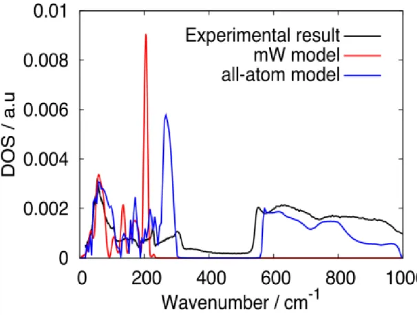
As will be shown below, the thermal expansivity is connected with the frequencies of the intermolecular vibrations via the Grüneisen parameter and the heat capacity. Therefore, some vibrational modes play a significant role in the appearance of its anomaly under cryogenic conditions. The distribution, known as the density of states (DOS), reveals the vibrational characteristics of ice. The calculated DOS resembles that of neutron scattering experiments, as shown in Figure 1 [9,31]. The DOS of the TIP4P/2005 model has two peaks. The modes in the lower frequency region of up to 400 cm−1 originate mostly from the translational motions, while the modes between 500 and 1000 cm−1 are associated mostly with the rotational (librational) motions. The frequency range of mW ice is limited to 250 cm−1 because all of the modes arise from the translational motions. The calculated DOS for TIP4P/2005 ice reproduces the overall feature of the experimental DOS. There are two distinct peaks in the low frequency region in both experimental and TIP4P/2005 ice.
The DOSs in the rotation-dominant region agree roughly with each other. The mW model also has two distinct peaks in the low frequency region. The peak position of the higher one is different from either of the other two. However, the position of the lower peak agrees with that of the TIP4P/2005 ice model and of the experimental one.
Since the modes in this low frequency region, which corresponds to the O-O-O bending, play a central role in giving rise to a negative thermal expansivity [6], the mW model or its variants could reproduce the negative thermal expansivity.
Figure 1. DOSs of ice Ic calculated with the mW model (λ = 23.15) and that of the all-atom model. The experimental neutron scattering data for ice Ih is also shown [31].
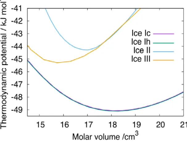
Although the mW model was developed for ice I, we attempt to use this model for other ice phases. The thermodynamic potential, A + pV, is plotted against the molar volume for several ice phases in Figure 2. The equilibrium molar volume, <V>, is the volume at which the thermodynamic potential is minimized. The equilibrium molar volume is reasonably obtained for ice Ic, Ih, II, and III. The curves of ices II and III reside totally inside the parabola of ice I, meaning that they cannot be the most stable phase at atmospheric pressure. When we elevate the pressure to 300 MPa, ice II and III can be stable relative to ice Ih with the mW model. We fail to obtain a smooth curve of the thermodynamic potential for ice VI. Probably, the deviation from the perfect tetrahedral coordination is too large to describe this ice structure through the mW model. The octahedral coordination of ice VII is also out of the applicable range of the force field model. The octahedral coordination does not mean that there are eight strong bonds for a molecule. It is impossible to distinguish four hydrogen bonding
molecules out of the eight neighbors in the mW model because of the absence of the hydrogen atoms. Another limitation is that the mW model cannot describe the difference between hydrogen-disordered ice and its hydrogen-ordered counterpart.
Thus, there is no way to distinguish, for example, ice Ih from ice XI.
Figure 2. Thermodynamics potential, A + pV, for several ice structures at
T = 20 K, obtained with the mW model. The curve for ice Ic overlaps completely with that of ice Ih.
The thermodynamic potential of Ic is the same as that of Ih for the mW model in the framework of the harmonic approximation, although Ih is slightly more stable than Ic experimentally. Because the interaction range is limited to the nearest four neighbors and they form an ideal tetrahedral arrangement both in ice Ih and Ic, no difference between them is expected for Uq at a fixed density. No practical difference in the vibrational free energy is found. The free energy from the anharmonic vibrations may give rise to the difference at high temperatures. Hereafter, we will not concern ourselves with the stability difference and will examine only ice Ic.
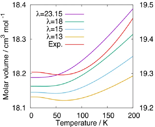
The equilibrium molar volume for ice Ic is plotted in Figure 3 as a function of temperature. It is evident that the thermal expansivity at low temperatures cannot be reproduced using the original mW model (λ = 23.15). In addition, the molar volume of 18.19 cm3 mol−1 is much smaller than the experimental value [3]. Figure 3 shows the volumes calculated with different λ values. We find that the negative thermal expansivity is successfully reproduced when the λ value is small enough, though only qualitatively.
Figure 3. Molar volume of ice Ic as a function of temperature for the mW model, calculated with several λ values. The molar volume of ice Ih from the experimental data is also shown (red, right axis) [3].
Figure 4. DOSs for ice Ic of the mW model with the original and modified λ values.
The equilibrium volume depends substantially on the tetrahedrality parameter, λ. A smaller λ makes the hydrogen bond network more flexible and leads to a more compact packing, while the tetrahedral coordination remains. As shown in Figure 4, the peaks in the DOS shift to a lower frequency as a result of the increase in flexibility due to the decrease in λ from 23.15 to 13. Figure 5 plots the thermal expansivity against the temperature. The critical λ value to recover the negative thermal expansivity lies around 18.
Figure 5. Thermal expansivities of ice Ic calculated using the mW model with λ= 23.15 (purple line), 18.00 (green line), 15.00 (cyan line), and 13.00 (yellow line).
2.4 Discussion
We calculate the temperature dependence of the molar volume for both the TIP4P/2005 model and the mW model. The purple curve in Figure 6 is the molar volume of ice Ic plotted against the temperature calculated with the all-atom TIP4P/2005 model. The value of 20.05 cm3 mol−1 is close to the experimental value for ice Ih, 19.3 cm3 mol−1 [3]. Figure 7 shows the thermal expansivity. The thermal expansivity of the TIP4P/2005 model is negative below 60 K, which is in agreement with the experimental result. We examine the effect of the coupling between the rotational and translational modes on the volume and its temperature dependence. The Hessian matrix, K, can be expressed as:
𝐊 = (𝐊𝑡𝑡 𝐊𝑡𝑟
𝐊𝑟𝑡 𝐊𝑟𝑟), (8)
where t and r denote the translational and rotational components, respectively.
We obtain a matrix Kb by removing the rotational-translational coupling elements, Ktr
and Krt.
𝐊𝑏 = (𝐊𝑡𝑡 0
0 𝐊𝑟𝑟), (9)
The thermodynamic properties without the rotational-translational coupling are calculated from the mode frequencies obtained by the diagonalization of the matrix Kb. Figure 6 shows that the volume of ice only slightly increases due to the removal of the coupling. However, the negative thermal expansivity disappears completely, as shown in Figure 7. It is also possible to eliminate the contributions from the rotational modes, as well as those from the rotational-translational coupling, by removing Krr in Equation 9. The volume calculated only from the translational motion is 19.38 3 cm3 mol−1, much smaller than the original value of the TIP4P/2005 model, 20.05 cm3 mol−1. Notwithstanding this, both the mW model and the TIP4P family reproduce the volume of liquid water fairly well [16], although there is a large discrepancy in the volume of ice I. The underestimation of the volume for the mW model may originate from the absence of the rotational modes. The shift to a higher frequency side upon compression in the TIP4P/2005 model is observed for the modes associated with the rotational motions, which is not shown but is a normal behavior against pressurization.
This causes a decrease in the volume.
Figure 6. Molar volume of ice Ic plotted against the temperature for the TIP4P/2005 model (purple), that calculated without the rotational- translational coupling (cyan), and that calculated only with the translational modes (green). The red curve is the volume of ice Ih from the experimental data. The volume of the mW model with λ = 13 is also shown (yellow, right axis).
Figure 7. Thermal expansivity of ice Ic plotted against the temperature for the TIP4P/2005 model (purple), that calculated without the rotational- translational coupling (cyan), and that calculated only with the translational modes (green). The red curve is the thermal expansivity from the experimental data [3]. The thermal expansivity of the mW model with λ = 13 is also shown (yellow).
The thermal expansivity, α, can be expressed as:
𝛼 =𝛾𝐶𝑣𝜅𝑇
3𝑉 , (10)
where γ is the Grüneisen parameter, 𝐶𝑣is the heat capacity, and 𝜅𝑇 is the isothermal compressibility. The Grüneisen parameter is expressed as:
𝛾 = ∑ 𝛾𝑖𝐶𝑖
𝑖
∑ 𝐶𝑖
𝑖
⁄ , (11)
where γi and 𝐶𝑖 are the Grüneisen parameter and heat capacity for the i-th mode, respectively.
The mode Grüneisen parameter of the i-th mode is defined as:
𝛾𝑖 = − (𝜕 ln 𝜈𝑖
𝜕 ln 𝑉). (12)
The heat capacity of a mode is given by:
𝐶𝑖 = 𝑘𝐵(ℎ𝜈𝑖 𝑘𝐵𝑇)
2
[exp (ℎ𝜈𝑖
𝑘𝐵𝑇) − 1]
−2
. (13)
Figure 8 shows the frequency dependence of the heat capacities of the vibrational modes defined as:
𝑐(𝜈) = ∫ ∑ 𝛿(𝜈′− 𝜈)𝐶𝑖𝑑𝜈′
𝑖 𝜈+∆𝜈
𝜈
, (14)
for the mW model with λ = 13 at three different temperatures. The heat capacity is almost zero for modes with frequencies higher than 80 cm−1 at T = 20 K, reflecting the fact that only very low-frequency modes can be thermally excited at such a low temperature.
Figure 8. Frequency dependence of the heat capacity of modes at temperatures 20 K (blue circle), 100 K (green diamond), and 400 K (red open square) for the mW model with λ = 13.
The mode Grüneisen parameter is calculated as follows. First, the mass- weighted Hessian matrix at the equilibrium volume, K0, is diagonalized as:
𝚲0 = 𝐔0†𝐊0𝐔0 , (15)
where Λ0 is the diagonalized matrix and U0 is the unitary matrix that diagonalizes K0. Next, the volume of the system is scaled isotropically by a factor of 1.0015, and the mass-weighted Hessian for the expanded system, Ke, is calculated. Similarly, the original system is scaled by 0.9985, and the mass-weighted Hessian for the shrunken system, Ks, is calculated. The mode frequencies of the expanded and the shrunken systems are calculated with the unitary matrix for the original volume:
𝚲𝑒 = 𝐔0†𝐊𝑒𝐔0 , (16) and
𝚲𝑠 = 𝐔0†𝐊𝑠𝐔0 . (17)
The differential value, γi, is numerically calculated from Λe and Λs. Figure 9 shows the frequency dependence of the product γiCi for the mW model with λ = 13.
The γi value is negative for the O-O-O bending modes around 50 cm-1. When the temperature is low enough, only this part contributes to the γ defined in Equation 11.
At higher temperatures, the positive contributions from the high frequency O-O stretching modes become dominant because of the increase in Ci. Therefore, the negative thermal expansivity is observed only at low temperatures. A similar result was reported for the TIP4P model [6].
Figure 9. Frequency dependence of γiCi at temperatures 20 K (blue circle), 100 K (green diamond), and 400 K (red open square) for the mW model with λ = 13.
As shown in Figure 5, the negative thermal expansivity is found for the mW model when the λ parameter is small enough. Figure 10 presents the frequency dependence of γi. The mode Grüneisen parameters are positive even in the region around 50 cm−1 for the original λ value of 23.15. This is probably because the modes around 50 cm−1 with the original λ value have a lower O-O-O bending character.
However, a decrease in the λ value can loosen the geometrical restriction of the arrangement on the three neighboring molecules and give rise to rather lower frequency modes, which may have the bending character.
Figure 10. Frequency dependence of the mode Grüneisen parameter for the original λ (blue circle), λ = 15 (green diamond), and λ = 13 (red open square).
2.5 Conclussions
We have calculated the chemical potential and volumetric properties of ice polymorphs with the original mW potential, applying the quasi-harmonic approximation. It is found that only several low-pressure ices (Ih, Ic, II, and III) are stable or metastable with the original mW model. The original mW model does not reproduce the negative thermal expansivity at low temperatures for ice I. A revision is proposed so as to recover the negative thermal expansivity. It is achieved by reducing one of the parameters of the force field model, λ, which was introduced for three molecules to favor the angle of the ideal tetrahedral arrangement, 109.47°. The origin of the negative thermal expansivity is examined for the revised mW model in terms of the anomalous mode Grüneisen parameters. In particular, the dependence of the mode Grüneisen parameters on the λ value is closely scrutinized. The magnitude of the negative mode Grüneisen parameters generally increases with decreasing λ value.
The calculated thermodynamic properties for mW ice are compared with those of a more realistic model, TIP4P/2005. The origin of the difference in the thermal expansivity is investigated by the chemical potential, whose vibrational free energy part is calculated from the block diagonal matrix in which all off-diagonal elements associated with translational-rotational degrees of freedom are removed. This decoupling of the translational and rotational motions eliminates the anomaly in the thermal expansivity and seems to be related to the observation that the negative thermal expansivity is not recovered with the original mW potential. The rotational degree of freedom may help to absorb the bare collisional motion between two adjacent oxygens through tight hydrogen bonding. The decrease in the λ value in mW, which loosens the geometrical restriction of the arrangement on the three neighboring molecules, seems to have a similar effect.
2.6 References
1. Dantl, G. Wärmeausdehnung von H2O- und D2O-Einkristallen. Zeitschrift für Physik 1962, 166, 115–118.
2. Röttger, K.; Endriss, A.; Ihringer, J.; Doyle, S.; Kuhs, W.F. Lattice constants and thermal expansion of H2O and D2O ice Ih between 10 and 265 K.
Addendum. Acta Crystallogr. B 2012, 68, 91.
3. Fortes, A.D. Accurate and precise lattice parameters of H2O and D2O ice Ih between 1.6 and 270 K from high-resolution time-of-flight neutron powder diffraction data. Acta Cryst. 2018, B74, 196–216.
4. Buckingham, D.T.W.; Neumeier, J.J.; Masunaga, S.H.; Yu Y.K. Thermal Expansion of Single-Crystal H2O and D2O Ice Ih. Phys. Rev. Lett. 2018, 121, 185505.
5. Fortes, A.D. Structural manifestation of partial proton ordering and defect mobility in ice Ih. Phys. Chem. Chem. Phys. 2019, 21, 8264–8474.
6. Tanaka, H. Thermodynamic stability and negative thermal expansion of hexagonal and cubic ices. J. Chem. Phys. 1998, 108, 4887–4893.
7. Grüneisen, E. Theorie des festen Zustandes einatomiger Elemente. Annalen der Physik 1912, 344, 257–306.
8. Nakamura, T.; Matsumoto, M.; Yagasaki, T.; Tanaka, H. Thermodynamic Stability of Ice II and Its Hydrogen-Disordered Counterpart: Role of Zero- Point Energy. J. Phys. Chem. B 2016, 120, 1843–1848.
9. Petrenko, V.F.; Whitworth, R.W. Physics of Ice; Oxford University Press:
Oxford, 1999.
10. Grimme, S. Semiempirical GGA-type density functional constructed with a long-range dispersion correction. J. Comput. Chem. 2006, 27, 1787–1799.
11. Pamuk, B.; Soler, J.M.; Ramìrez, R.; Herrero, C.P.; Stephens, P.W.; Allen, P.B.; Fernàndez-Serra, M.-V. Anomalous Nuclear Quantum Effects in Ice.
Phys. Rev. Lett. 2012, 108, 193003.
12. Salim, M.A.; Willow S.Y.; Hirata, S. Ice Ih anomalies: Thermal contraction, anomalous volume isotope effect, and pressure-induced amorphization. J.
Chem. Phys. 2016, 144, 204503.
13. Gupta, M.K.; Mittal, R.; Singh, B.; Mishra, S.K.; Adroja, D.T.; Fortes, A.D.;
Chaplot, S.L. Phonons and anomalous thermal expansion behavior of H2O and D2O ice Ih. Phys. Rev. B 2018, 98, 104301.
14. McKinley, J.L.; Beran, G.J.O. Identifying pragmatic quasi-harmonic electronic structure approaches for modeling molecular crystal thermal expansion.
Faraday Discuss. 2018, 211, 181–207.
15. Abascal, J.L.F.; Vega, C. A general purpose model for the condensed phases of water: TIP4P/2005. J. Chem. Phys. 2005, 123, 234505.
16. Sanz, E.; Vega, C.; Abascal, J.L.F.; MacDowell, L.G. Phase Diagram of Water from Computer Simulation. Phys. Rev. Lett. 2004, 92, 255701.
17. Aragones, J.L.; Vega, C. Plastic crystal phases of simple water models. J.
Chem. Phys. 2009, 130, 244504.
18. Hirata, M.; Yagasaki, T.; Matsumoto, M.; Tanaka, H. Phase Diagram of TIP4P/2005 Water at High Pressure. Langmuir 2017, 33, 11561–11569.
19. Yagasaki, T.; Matsumoto, M.; Tanaka, H. Phase Diagrams of TIP4P/2005, SPC/E, and TIP5P Water at High Pressure. J. Phys. Chem. B 2018, 122, 7718–
7725.
20. Jorgensen, W.L.; Chandrasekhar, J.; Madura, J.D.; Impey, R.W.; Klein, M.L.
Comparison of simple potential functions for simulating liquid water. J. Chem.
Phys. 1983, 79, 926–935.
21. Ramírez, R.; Neuerburg, N.; Fernández-Serra, M.-V.; Herrero, C.P. Quasi- harmonic approximation of thermodynamic properties of ice Ih, II, and III. J.
Chem. Phys. 2012, 137, 044502–044513.
22. Molinero, V.; Moore, E.B. Water modeled as an intermediate element between carbon and silicon. J. Phys. Chem. B 2009, 113, 4008–4016.
23. Jacobson, L.C.; Hujo, W.; Molinero, V. Nucleation pathways of clathrate hydrates: effect of guest size and solubility. J. Phys. Chem. B 2010, 114, 13796–13807.
24. Moore, E.B.; Molinero, V. Ice crystallization in water’s “no-man’s land.” J.
Chem. Phys. 2010, 132, 244504.
25. Stillinger, F.H.; Weber, T.A. Computer simulation of local order in condensed phases of silicon. Phys. Rev. B 1985, 31, 5262–5271.
26. Laradji, M.; Landau, D.P.; Dünweg, B. Structural properties of Si1-xGex alloys:
A Monte Carlo simulation with the Stillinger-Weber potential. Phys. Rev. B Condens. Matter 1995, 51, 4894–4902.
27. Takenaka, K. Negative thermal expansion materials: technological key for control of thermal expansion. Sci. Technol. Adv. Mater. 2012, 13, 013001.
28. Fabian, J.; Allen, P.B. Thermal expansion and Grüneisen parameters of amorphous silicon: A realistic model calculation. Phys. Rev. Lett. 1997, 79, 1885.
29. Moore, E.B.; Molinero, V. Structural transformation in supercooled water controls the crystallization rate of ice. Nature 2011, 479, 506–508.
30. Matsumoto, M.; Yagasaki, T.; Tanaka, H. GenIce: Hydrogen-Disordered Ice Generator. J. Comput. Chem. 2018, 39, 61–64.
31. Li, J. Inelastic neutron scattering studies of hydrogen bonding in ices. J. Chem.
Phys. 1996, 105, 6733–6755.
Chapter 3
On the Study of Solubility of Gas Molecules in Clathrate Hydrate
3.1 Introduction
Clathrate hydrates are non-stoichiometric compounds consisting of guests and the water molecules. The tetrahedrally hydrogen-bonded water molecules form firm cages structures made of planar hexagon and pentagon in which the guest molecules are incorporated. In that sense, the properties of the empty clathrate hydrates resemble low-pressure hexagonal ice (Ice Ih). In fact, the negative thermal expansivity in ice Ih at low temperature is observed in metastable ice XVI, which is a disguised form of clathrate hydrate structure having no guest form[1,2]. However, ice Ih gas only puckered rings while clathrate hydrate has planar rings to form 12-to 16 hedra. The guest molecules in hydrate cage are divided into four groups: 1) hydrophobic gases such as methane, 2) water-soluble gases polarized weakly such as carbon dioxide, 3) water-soluble polar compounds. Other than those clathrate hydrates in which guest species do not participate in the host structure, guest molecules can be a part of the host site, which is known as semi-clathrate hydrate containing water-soluble ternary or quaternary alkyl-ammonium salt. The thermodynamic stability of clathrate hydrate relies totally on the presence of guest molecules. Without such gases inside the hydrate cage, the structure is at most metastable[3].
There are three clathrate hydrates structures occurring in nature: cubic structure I (sI) mostly found encaging intermediate size of guests, structure II (sII) mostly containing small or large guests and hexagonal structure (sH) that is present with both small and large guest molecules simultaneously[4]. The sI structure consists of 512 and 51262 cages accommodating methane, ethane and carbon dioxide, the sII structure
![Table 1. Parameters of the mW model [22].](https://thumb-ap.123doks.com/thumbv2/123deta/5814910.1033633/26.892.186.757.351.679/table-parameters-mw-model.webp)