WORKING PAPER SERIES
ugust 2002 Working Paper No.74
Government Deficit, Public Investment and Public Capital
in the Transition to an Aging Japan by
Ryuta Ray Kato
August 2002
Faculty of Economics
SHIGA UNIVERSITY
1-1-1 Banba, Hikone, SHIGA 522-8522, JAPAN
Government De…cit, Public Investment
and Public Capital in
the Transition to an Aging Japan
(A Full Version)
August 2002
Ryuta Ray Kato
Faculty of Economics Shiga University, Japan
and
Management School Imperial College, UK
Forthcoming in
Journal of the Japanese and International Economies
———————————————————————————
This is a full version of the paper. The version appearing in Journal of the Japanese and International Economies is a digest version due to a limited space in the Journal. I would like to thank all the participants at 14th NBER conference held in Tokyo in December 2001. I would also like to thank Makoto Saito and Takeo Hoshi for their valuable comments and suggestions at the NBER conference. Constructive suggestions by a referee are also appreciated.
Government De…cit, Public Investment
and public capital in the Transition
to an Aging Japan
August 2002 Ryuta Ray KatoAbstract
This paper tires to examine the e¤ects of government de…cits, public investment, public capital and public pension policies on the tax burden, capital accumulation and economic welfare in the transition to an aging Japan by applying a simulated method in the expanded life cycle general equilibrium growth model.
One of the main results of this paper is that the highest income, thus the highest economic growth, is achieved when the future government de…cits are the highest. However, such a policy to achieve the highest economic growth with the highest government de…cits is necessarily not most preferable for future generations, since disposable income under this policy is necessarily not the highest due to the reason that a drastic increase in a consumption tax rate has to be followed in the future to …nance the huge amount of interest payments. Thus, only targeting high economic growth would mislead us as to the economic policy. The implication of this result is that a policy to reduce the future government de…cits is most preferable for almost all generations, even though a cut in the future de…cits must be followed by a decrease in public investment, thus a decrease in the future public capital.
By proposing three di¤erent scenarios regarding the future government de…cit policy, this paper also presents numerical results of the e¤ects on future consumption tax rates, tax burdens, social security burdens, and the generational accounting through the existing pay-as-you-go public pension scheme.
The e¤ects of an introduction of technological progress as well as of ine¢ciency in public investment will also be examined numerically.
JEL Classi…cation: H55, H54, H62, C68, J10 Keywords:
Government De…cits, Public Investment, Public Capital, Aging Population, Over-lapping Generations Model, Public Pension Scheme, Simulation
Correspondence: Ryuta Ray Kato
Faculty of Economics, Shiga University 1-1-1 Banba, Hikone, Shiga 522-8522 Japan
Phone&Fax: +81-(0)749-27-1070 (direct)
1 Introduction
This paper tries to examine the e¤ects of future government de…cits, public investment and public capital on the tax burden, capital accumulation and economic welfare in the transition to an aging Japan by applying a simulated method in the expanded
life cycle general equilibrium growth model.1
Economic policies, speci…cally such as government debt policies, the future sched-ule of public investment, or the reform of a public pension scheme, should be evaluated intertemporally, since these policies involve redistributional e¤ects on di¤erent gen-erations. On one hand, bene…ts from public capital generated by public investment are partly transferred for a long time to future generations from current generations if public investment is …nanced by taxes imposed on current generations. On the other hand, issuing government bonds is the way to avoid to pay de…cits of current generations back, and thus bene…ts are transferred from future generations to current generations, since an increase in government de…cits must be followed by an increase in taxes imposed on future generations.
In the past, the huge amount of the existing public capital was used to be …nanced by issuing government bonds in Japan. If intergenerational e¤ects of government debt policies of Japan are considered, public capital …nanced by issuing government bonds should also be taken into account to measure the net re-distributional e¤ect of debt policies among di¤erent generations.
Furthermore, it is forecasted that Japan will become an aged society quite rapidly. An aging population implies an increase in the contribution to a public pension scheme provided that the existing pay-as-you-go scheme is maintained in Japan, thus, result-ing in further burdens on future generations. An agresult-ing population induces transfers of bene…ts from current generations to future generations if the existing pay-as-you-go scheme is unchanged, and the future demographic change should also be taken into
account.2 Thus, if an intergenerational aspect of future government policies is
exam-1This paper expands Kato (2000, 2002b) by incorporating public capital into the model and
re-examines the e¤ects of the future Japanese government debt policy by presenting several scenarios.
gen-ined, these three channels (government de…cits, public pension scheme, and public capital) must be comprehensively considered.
In the transition to an aging society, the e¤ects of government policies are di¤erent among each future generation, as pointed out by Auerbach and Kotliko¤ (1987). An insight can only be given by numerical examinations if future policies are examined speci…cally in the transition to an aging society. A simulated method based on the actual and forecasted data could give us as real evaluation of future government policies as possible. Numerical results could also be used to evaluate the ongoing structural reform facing the Japanese government.
It is generally evaluated that higher economic growth is more desirable, since higher economic growth results in higher income. An economic policy which induces higher economic growth in the long run is thus more preferable. However, since eco-nomic policies have di¤erent e¤ects among future generations, the evaluation might not be straightforward, if the policies are examined intergenerationally. Furthermore, economic policies should ultimately be evaluated based on utility of di¤erent gen-erations. In this paper, two measures will be given to evaluate future government debt policies: Economic growth at each time in the future and equivalent variation of lifetime utility of each generation. The latter corresponds to the overall evaluation of intertemporal government policies based on utility of each generation.
One of the main results of this paper is that a government de…cit policy which achieves the highest income in a steady state is necessarily not most preferable, if the policy is evaluated on lifetime utility. The highest income is achieved when the future government de…cits are the highest. Since future generations save more, expecting a drastic increase in a consumption tax rate in order to …nance the huge amount of interest payments incurred from outstanding bonds in the future, higher government de…cits induce more savings, thus, resulting in more supply of capital. The increase in the supply of capital induces higher income, and thus the highest economic growth can be achieved when the future government de…cits are the highest. However, when erations to future generations, the net transfer is zero between current and future genrations. It depends on the magnitude of bequest motives, and it is still true that a pay-as-you-go scheme transfers bene…ts from current to future generations in an aging society.
the future government de…cits are the highest, the consumption tax rate is also the highest in the future, which implies that disposable income is necessarily not the highest. Thus, lifetime income is necessarily not the highest, and such a policy is not preferable if the policy is evaluated on utility, even though pre-taxed income is the highest. This result suggests that only targeting high economic growth would mislead us as to the economic policy.
This paper is organised as follows: Section 2 presents the feature of this paper by referring to the related literature and Section 3 presents the basic model employed in the simulation analysis. Section 4 shows the method of the simulation analysis and its assumptions. Section 5 evaluates the e¤ects of future government de…cit policies, and Section 6 examines the e¤ect of an introduction of technological progress as well as of ine¢ciency in the future public investment. Section 7 summarizes and concludes the paper.
2 The Feature of this Paper
2.1 The Related Literature
There are three …elds in the literature related to this paper: The Japanese government de…cit, public capital in Japan, and the public pension scheme in an aging Japan. 2.1.1 The Japanese Government De…cit
The e¤ects of the Japanese government debt policy have been discussed in di¤erent ways. However, an intergenerational aspect of government de…cits has not been stud-ied in detail, since their main concerns were with the evaluation of the past policies or the sustainability of the Japanese government debt policy by using the past actual data, where econometric methods were mainly used rather than simulated methods. Their concerns were in the test of the tax smoothing hypothesis presented by Barro (1979) and the test of the sustainability of the Japanese debt policy. In the former, Asako et al (1993) and Nakazato (2000) are categorized. Asako et al (1993) tested
the hypothesis by the Phillips and Perron unit-root test, the Cochrane statistics, and Hall’s (1978) test. Nakazato (2000) tested the hypothesis by Campbell’s (1987) test. Both papers pointed out that there was a possibility for the past Japanese govern-ment debt policies to be made based on other aspects such as political power than tax smoothing. In the latter, Asako et al (1993), Fukuda and Teruyama (1994), Kato (1997), Doi and Nakazato (1998) and Doi (2000) are categorized.. They used dif-ferent equations for tests, and have not come to the same conclusion regarding the sustainability of government de…cits in Japan. There are also papers based on a sim-ulated method to examine Japanese government de…cits. Kawagoe (2000) recently presented several proposals by simulating the e¤ect of government de…cit policies of Japan based on OECD …gures. Kato (2000, 2002a, 2002b) examined the e¤ects of the future government de…cits on future generations by presenting several scenarios. The main di¤erence of this paper from Kato (2000, 2002b) is an incorporation of pub-lic capital to comprehensively explore the e¤ects of the future government popub-licy on future generations. This paper is also di¤erent from Kato (2002a) in the future pop-ulation data used in the simpop-ulation. This paper uses the latest version of the actual forecasted population data estimated in 2002 by the National Institute of Population and Social Security Research, which was not available in Kato (2002a). Nothing is more natural in a simulation analysis than using the latest available data which is as realistic as possible.
2.1.2 Public Capital in Japan
Since Aschauer (1989a, 1989b), there have been several papers to estimate the e¤ect of public capital in Japan. Their main concerns were related to the examination of the e¤ect of public investment in Japan. Iwamoto (1990) discussed the socially optimal level of public investment in Japan, which is based on Arrow and Kurz (1970), and he estimated that the existing level of public capital would be lower than the optimal level. Doi (1995) also estimated the optimal level by using the data of local as well as urban areas and he concluded that the public capital in local (urban) areas would be higher (lower) than the optimal level due to the heterogeneity of
political power in di¤erent areas. Asako and Sakamoto (1993), Asako et al (1994), Ogawara and Yamano (1995), and Yoshino and Nakano (1994, 1996) estimated the e¤ect of public capital on production of the private sector. These econometric results of the e¤ect of public capital on the private sector production are well summarised in
two excellent books by Yoshino and Nakajima (1999) and Mitsui and Ohta (1995)3.
Their concerns were with the estimation of parameters regarding the stock of public
capital in the private sector production function4, and the estimated parameters will
be used in this paper to examine the e¤ect of the public capital stock. Kato (2002a) explicitly incorporated public capital into the overlapping generations model in order to evaluate the e¤ect of the future government de…cit policy on di¤erent generations. 2.1.3 The Existing Public Pension Scheme in an Aging Japan
The e¤ects of an aging population, and/or the e¤ects of several tax policies and public pension policies in the transition to an aging Japan have been discussed by applying simulated overlapping generations models in the literature. A simulated Overlapping Generations Model originated by Auerbach and Kotliko¤ (1983) was …rst applied to the analysis of the e¤ect of tax policies and public pension policies of Japan by Homma et al (1987), and the existing studies have expanded Auerbach/Kotliko¤ model to discuss several government policies in the transition to an aging Japan (Iwamoto (1990a), Iwamoto et al (1991 and 1993), Atoda and Kato (1993), and Kato (1998)). Hatta and Oguchi (1999) recently emphasized intergenerational redistribu-tion of income through the public pension scheme by applying their own simulated method. Kato (2000, 2002a, 2002b) expanded Kato (1998) by incorporating gov-ernment de…cits into the model. In Japan the existing public pension scheme is a modi…ed pay-as-you-go scheme, where a certain amount of fund is accumulated at the same time. This accumulated fund is supplied in the capital market, and the total
3See also Prof Doi’s excellent web at http://www.econ.keio.ac.jp/sta¤/tdoi/ for the survey of the
literature.
4An exception is Akagi (1996), where an aspect of public capital to improve utility such as public
parks was considered under the assumption that the stock of utility related public capital is one of elements in utility.
sum of government bonds and the accumulated fund in the public pension scheme is the net real amount of government debts. Thus, the e¤ect of government de…cits should be discussed by taking into account the existing public pension fund. Kato (2000, 2002b) expanded Kato (1998) in the following two aspects: The one aspect was that in the simulation analysis of Kato (2000, 2002b) the later version of the actual forecasted population data estimated in 1997 by the National Institute of Population and Social Security Research was used. The other aspect was the explicit incorpora-tion of government de…cits into the model. Since the main concern of Kato (1998) was to discuss the e¤ect of the transition of an aging population in Japan through the existing public pension scheme, little attention was paid to the e¤ect of outstanding government debts in Japan.
2.2 The feature of this paper
The key feature of this paper is to explicitly incorporate public capital into Kato (2000, 2002b). In Japan the huge amount of the existing public capital was …nanced by issuing government bonds in the past. Since the bene…ts from the existing public capital is partly transferred for a long time to future generations, the Japanese gov-ernment debt policy have to be evaluated by taking into account the e¤ect of public capital on future generations, if the intergenerational e¤ect on the past as well as on the future generations is considered. In the simulation of this paper, the past actual data of the public capital stock is used in order to make key parameters realistic.
This paper is also di¤erent from Kato (2000, 2002b) in the treatment of taxes. Apart from a consumption tax, a wage tax was also considered in Kato (2000, 2002b) as a tool to …nance the future shortage of money. However, the e¤ect of consumption taxation is only taken into account in this paper. This is not because consumption taxation is more preferable or plausible, but because it involves more complicated e¤ects, which are often di¢cult to be analyzed in a completely theoretical setting. In a simulation analysis under realistic assumptions, the di¢culty can numerically be overcome, and more realistic implication regarding the e¤ect of the future gov-ernment debt policy can be drawn. The change of a consumption tax rate induces
tax distortion, which consists of a substitution e¤ect as well as an income e¤ect. If the goods are normal, these two e¤ects function oppositely to each other, and thus, the overall e¤ect can usually not be determined analytically. However, when labor is assumed to be exogenously given, the e¤ect of the change of a wage tax rate is straightforward as long as the goods are normal, since there is no substitution e¤ect. In this paper, labor is assumed to be exogenously given, and a consumption tax is only considered in order to deepen the analysis by changing several assumptions such as the degree of technological progress and the degree of e¢ciency in future public investment.
The di¤erence of this paper from Kato (2002a) is in the future population data used in the simulation. In Kato (2002a) the low variant future population data estimated in 1997 was used. In this paper the latest version of the medium variant future population data estimated in 2002, which was not available in Kato (2002a), is used. The low variant estimation in the version of 1997 estimation was most predictable, and the medium variant estimation in the latest version estimated in 2002 is the closest to the most predictable estimation in 1997. Thus, in this paper the medium variant estimation in the latest version by the National Institute of Population and Social Security Research is used in the simulation analysis.
3 The Model
In an economy, where time is assumed to be discrete every year, there are three types of agents, households, …rms, and a government. The behaviour of each agent is described as follows:
Households:
Each generation is assumed to have the same income, mortality rate, and utility function. It is also assumed that each generation appears in the economy as a decision making unit at the age of 21 and live to a maximum of 100 with a certain probability
of death for every period. When qj +1;j is the conditional probability that a household
until s + 21 can be expressed as
Ss=
sY¡1
j=1
qj+1;j;
where qj+1;j is calculated from the actual data estimated by the National Institute
of Population and Social Security Research in 2002. Assuming that each household makes lifetime decisions about the allocation of wealth between consumption and savings in order to maximise its expected utility, the expected utility at age s + 20 would be U = 80 X s=1 Ss(1 + ±)¡(s¡1) C1¡ 1 ° s 1 ¡ 1 ° ; (1)
where Csrepresents consumption at age s+20; ± the discount rate, and ° the elasticity
of intertemporal substitution. As expressed in (1), it is assumed that there are no
bequest motives for simplicity.5
It is assumed that each household at age s + 20 has the budget constraint such that
As+1 = [1 + (1 ¡ ¿r(t)) r (t)] As+ (1 ¡ ¿y(t) ¡ ¿p(t)) w (t) es
+bs+ as¡ (1 + ¿c(t)) Cs; (2)
where As represents the amount of assets held by each household at the beginning
of age s + 20, r (t) is the interest rate at period t, es is the e¢ciency unit of labor
which depends on age, and w is the wage rate per e¢ciency unit of labor.. For the sake of brevity, the labor supply is assumed to be inelastic and the labor supply after retirement is assumed to be zero. For the estimation of the e¢ciency unit of labor
es, the following equation has been estimated:
e = a0+ a1A + a2A2+ a3L + a4L2;
where A represents age, L the length of employment, and e the wage rate per hour, respectively. The above equation has been estimated under the assumption that
5This assumption is only for simplicity. However, as has kindly been suggested by Makoto Saito,
workers do not change their jobs during their working periods.6
All tax systems are based on proportional taxation, with ¿y representing the wage
income tax rate, ¿r the interest income tax rate, ¿cthe consumption tax rate, and ¿p
the contribution to the public pension scheme. In order to re‡ect the actual aspect of the existing public pension scheme in Japan, 1/3 of the total amount of the public
pension bene…ts is assumed to be …nanced by taxes. as is the expected amount of
post-taxed bequests to be inherited. It is assumed that there is no private pension
market. For simplicity bequests are assumed to be inherited at age 50.7 b
s is the
amount of public pension bene…ts, which is assumed such that
bs = ÁH (s ¸ RP ) bs = 0 (s < RP ) ; H = 1 IR IR X s=1 w (t) es;
where Á and H denote the replacement ratio and the average annual remuneration, respectively. RP +20 and IR +20 denote the age at which households start to receive public pension bene…ts and the retirement age, respectively. Since the actual public pension system in Japan is a double indexation system, the above assumptions are only for simplicity.
Furthermore, the following two constraints are incorporated in addition to the conventional budget constraint. The …rst constraint is one the consumption level such that
Cs¸ CMIN; (3)
6This implies that it might have an upward bias. However, the author does not believe that this
bias would be crucial for the aim of this paper.
By using the data from ”The Investigation of the Wage Structure (Chingin Kozo Kiso Chosa) in 1994,” the above variables have been estimated as
a0 a1 a2 a3 a4
¡0:1537 0:05539 ¡0:0007595 0:1045 ¡0:001901
(¡0:5363) (2:865) (¡4:019) (4:823) (¡3:243)
7Several patterns of the timing when bequests are inherited have been examined in Atoda and
where CMIN denotes the minimum consumption level. The other constraint is the households’ liquidity constraint. Considering the inaccuracy of lifetime in the model, the households are apt to see their public pension bene…ts, which they will receive from the age 65, as security and produce a high level of consumption when they are young, since the weight placed on consumption at old age is extremely reduce due to their uncertainty of their lifetimes, resulting in a very small amount of consumption when they are old. However, in reality the public pension bene…ts cannot actually o¤er security. Given that the assets at the end of each previous period are negative, a liquidity constraint is imposed on consumption at the present period in this way:
Cs · [1 + (1 ¡ ¿r(t)) r (t)] As+ (1 ¡ ¿y (t) ¡ ¿p(t)) w (t) es+ bs+ as
´ DYs: (4)
Now, suppose that each household maximises its utility under these constraints, and the maximization of (1) subject to (2), (3), and (4) yields (see Appendix for the detailed deduction) Cs = µ ANCs£ C ¡1 ° 1 + AOBs ¶¡° ; (5) where ANCs = ANB (t) S1(1 + ±)(s¡1) Ss ; ANB (t) = P C (t) P C (1)Q80t=1ARA (t); P C (t) = 1 + ¿c(t) ; ARA (t) = 1 + (1 ¡ ¿r(t)) r (t) ;
and P C (1) expresses P C (t) of households at age 21: AOBs is given by:
AOBs = (1 + ±)(s¡1) Ss 8 > > > > > < > > > > > : ANB (t) 2 6 4 Á11¡ Á21¡ P C (1)P80s=2Á2sDYs³Qst=1¡1ARA (t) ´ 3 7 5 +Á2s¡ Á1s 9 > > > > > = > > > > > ; :
From (5), the optimal consumption behaviour of all ages can be derived if the
initial consumption C1 is speci…ed, and the savings level can be calculated from (2)
Firms:
A main di¤erence from Kato (2000, 2002b) is in the assumption of a production function. In this paper it is assumed that the public capital stock a¤ects the private sector production as follows:
Y (t) = ª (t) K (t)®L (t)1¡®G (t)¯; (6)
where K (t) represents the private capital, L (t) the labor supply measured by the e¢ciency unit, and G (t) the public capital stock, respectively. Note the di¤erence between age, generation, and period. Denoting the generation by I, the age s, and the period t, they are related to each other such that t = I + s ¡ 1:
ª (t) denotes the scale parameter, which is also interpreted as the measure of technological progress. As assumed in (6), the total output is distributed to the private capital and the labor, and the complicated consideration of the return to the government is excluded. The value of ¯ is given by the latest estimation by Yoshino and Nakajima (1999) in order to examine the scale of the e¤ect of public capital on output in the transition to an aging Japan.
From the pro…t maximization of …rms subject to (6), the …rst-order condition is derived to be: w (t) r (t) = 1 ¡ ® ® Ã K (t) L (t) ! :
The property of a constant-return-to-scale production function with respect to the labor and the private capital yields
Y (t) = w (t) L (t) + r (t) K (t) :
Government:
Suppose that the government consists of a narrower government sector and a public pension sector. A narrower government sector is assumed to spend revenue on general government expenditure. The narrower government sector consists of central as well as local governments expenditure, transfers and the expenditure on public investment. A 1/3 of the total amount of the public pension bene…ts is assumed to be transferred from the account of the narrower government sector to the account of
the public pension sector. The budget of the narrower government sector is assumed to be …nanced by collecting taxes as well as issuing government bonds. The budget constraint on the narrower government sector at time t is given by:
D (t + 1) ¡ D (t) = GE (t) + r (t) D (t) + P en (t) ¡ R (t) ;
where D (t), R (t), and GE (t) denote the amount of outstanding government debts, total tax revenue and general government expenditure at time t, respectively. P en (t) is the amount of the transfer from the narrower government sector to the public pension sector. The budget constraint on the public pension sector is given by:
F (t + 1) ¡ F (t) = r (t) F (t) + P en (t) + P (t) ¡ B (t) ;
where F (t), B (t) and P (t) denote the amount of the public pension fund, total public pension bene…ts, and the total amount of the contribution to the public pension scheme, respectively. R (t), P (t) and B (t) are given by
R (t) = ¿y(t) w (t) L (t) + ¿r(t) r (t) AS (t) + ¿c(t) AC (t) + ¿h(t) BQ (t) ; P (t) = ¿p(t) w (t) L (t) ; B (t) = 80 X s=45 SsNsbs;
where ¿hand Nsdenote the inheritance tax rate and the sum of s-year-old generations
at time t, respectively. AS (t), AC (t) and BQ (t) denote the total amount of savings, consumption and bequests inherited by the generation of age 50 in the economy at time t; respectively, and given by
AS (t) = 80 X s=1 SsNsAs; AC (t) = 80 X s=1 SsNsCs; BQ = 80 X s=1 (1 ¡ Ss) NsAs: Market Equilibrium:
A equilibrium condition in the capital market is given by AS (t) + F (t) = K (t) + D (t) ;
and in the goods market it is
Y (t) = AC (t) + K (t + 1) ¡ K (t) + GE (t) :
4 Assumptions in the Simulation
4.1 Structure and Data
In order to examine the e¤ects of changes in the demographic structure caused by the transition to an aging population, especially when applying the simulated method, it is most natural to use population data which are as realistic as possible. Using the latest actual population data estimated in 2002 by the National Institute of Population and Social Security Research, this paper has succeeded in reproducing these data exactly by applying the model constructed in Section 3. The demographic structure in this model has been generated by the following procedure.
4.1.1 Population Structure
All generations born before the generation of age 100 in 1990 (the generation born in 1890) are assumed to have the same birth and mortality rates as the generation of age 100 in 1990, so that the demographic structure of all generations born before 1890 is identical. It is also assumed that the population distribution will continue to be the same for each period from year 2100. Based on these assumptions, the actual future population data estimated in 2002 by National Institute of Population and Social Security Research have been used for the periods from year 2001 to 2100 and the actual population data in ”Population Census of Japan (Kokusei-chosa)” for the periods before 2001.
For the period prior to 2001, whenever the actual data from the Population Census of Japan (Kokusei-chosa), which is held every …ve years, was not available, actual population data from the ”Simple Static Life Table” (from the Japanese Ministry of Health and Welfare) were used. The estimated number of people at the age of 100 for the periods from 2001 to 2100 has been calculated by using the data on
survival probabilities based on sex and age from the estimation made in 2002 by the National Institute of Population and Social Security Research. Such assumptions for the demographic structure were made due to the fact that the latest actual data available were those of 2000 and the estimation made in 2002 by National Institute of Population and Social Security Research only covers the periods from 2001 to 2100. The following point regarding the future population data should also be noted: In this paper the medium variant estimation has been used. This is because the low variant future population data in the previous version estimated in 1997 was most predictable and the medium variant estimation in the latest version estimated in 2002 is the closest to the most predictable low variant estimation in 1997. Thus, in this paper the medium variant estimation in the latest version by the National Institute of Population and Social Security Research has been used in the simulation analysis, since nothing is more natural in a simulation analysis than using the latest available data which is as realistic as possible.
In Table 2 the total population, the population between age 15 and 64, and the
population of age 65 and over are shown8. The aging rate, which is de…ned as the
ratio of the population of age 65 and over to the total population, is also shown in Table 2.
All parameters in this paper have been set so that the economic variables obtained from the actual Japanese data of 1997, such as the ratios of certain tax revenues to the total tax revenues, could be reproduced as exactly as possible. In other words, the induced estimation data of 1997 from the simulation analysis has been set as close as possible to the real Japanese data of 1997.
8The number of labor force is usually de…ned as the number of the employed and the unemployed
of age 15 and over, and thus the population between age 15 and 64 is exactly not the same as the number of labor force. However, since the number of labor force in terms of the future population cannot be obtained, the population between age 15 and 64 of future generations can correspond to the number of labor force in the future. The population of age 65 and over shown in Appendix 2 is the number of recipients of the public pension scheme.
4.1.2 Outstanding Government debts and Public Pension Fund
The actual data of outstanding governments debts has been used until 1999, and the actual data of the public pension fund has been used until 1998. It is assumed that the public pension scheme started in 1956. The data consists of central government debts
and local governments debts9. The actual GDP data has also been used until 1999.
Since the main purpose of this paper is to explore the e¤ect of future government de…cits, the future value of the pubic pension fund-GDP ratio is assumed to be the same in all scenarios, as shown in Figure 1. It has been assumed that the future ratio of the public pension fund to GDP converges to the same value in all cases in a steady state under the assumption that the growth rate of the future ratio decreases through time until the growth rate becomes zero. The shortage of money spent in a public pension sector in each scenario is assumed to be …nanced all by an increase in the
contribution rate ¿p. The replacement ratio in the public pension scheme is assumed
to be 56% in all scenarios. The debt-GDP ratio and the public pension fund-GDP ratio prior to 1998 are actual ratios in this paper. Note that the actual values of the debt-GDP ratios in this paper are de…ned based on the actual outstanding levels of central and local governments debts, and thus they are not the same as the OECD values, where outstanding local government debts are not included.
Regarding the future debt-GDP ratio, the following three cases have been con-sidered in this paper: The ratio of outstanding government debts to GDP (the D-G ratio) converges to a 120 % level in Case 1, a 150 % level in Case 2, a 90 % level in Case 3, respectively. The detailed values are given in Table 3. Note that the future values are also de…ned based on the level of outstanding central and local governments debts.
Narrowed or widened government de…cits are always followed by an increase or a decrease in tax rates. Thus, when the e¤ects of future government de…cit policies are explored, a tax associated with future government de…cit policies must be speci…ed.
9The actual data of outstanding central government debts has been obtained from Budget
Sta-tistics (Zaisei Tokei) and that of outstanding local governments debts from Annual Report on Local Governments Bonds (Chihosai Tokei Nenpo).
In this paper a consumption tax has been used in each case10. It has also been assumed that a policy change occurs in 2003: Until 2002 the consumption tax rate is …xed and the wage tax rate is endogenously calculated in each scenario. The …xed consumption tax rates until 2002 have been given, taking into account the actual aspect of consumption taxation in Japan so that they have been set at 2 % before 1989, 5 % from 1990 to 1994, and 7 % from 1995 to 2002. After 2003 the consumption tax rate is endogenously obtained under the assumption that the wage tax rate remains at the level of 2002.
<Case 1: 120 % D-G Ratio>
The growth rate of the D-G ratio decreases until the D-G ratio converges to a 120 % level in a steady state. The shortage of money spent in a narrower government sector is assumed to be …nanced by a consumption tax after 2003. This case corre-sponds to a current debate that maintaining the D-G ratio at a 120 % level would be most reasonable.
<Case 2: 150 % D-G Ratio>
A steady state level of the D-G ratio is assumed to converge to a 150 % level. The shortage of money spent in a narrower government sector is assumed to be …nanced by a consumption tax after 2003. This case corresponds to the most possible situation the Japanese government is currently facing.
<Case 3: 90 % D-G Ratio>
A steady state level of the D-G ratio is assumed to converge to a 90 % level, which is lower than the current level (year 1999). The shortage of money spent in a narrower government sector is assumed to be …nanced by a consumption tax after 2003. This case takes into account a rapid increase in the growth rate of the D-G ratio in the past 3 years. This case corresponds to another debate that the Japanese government should decrease the amount of public investment to reduce future government de…cits.
4.1.3 General Government Expenditure
General government expenditure has been assumed to consist of central and local governments consumption, public investment and transfers. The transfer to a public pension sector is not included in this category. The actual data until 1999 has been used in this paper. It has been assumed that in all scenarios governments consumption and transfers partly grow at the same rate as the growth rate of an aging population. The growth rates have been given based on the following assumptions: The average ratio of transfers to the elderly to the total transfers through an account, which is speci…c to the elderly, in the public health insurance scheme in the past 10 years is 33.4 %. Thus, it has been assumed in this paper that a 33.4 % of governments consumption and transfers grows at the same rate as an aging population in the future. The detailed values are presented in Table 4.
4.1.4 Public Investment
Public investment in the future has been assumed to depend on the future government debt policy, since a certain amount of pubic investment has been …nanced by issuing construction bonds in the past. In the last …fteen years from 1984 to 1998, the ratio of public investment to outstanding government debts is quite stable around 12.75 %. In this paper it has been assumed that the ratio does not change in the future. Being based on this assumption, the future values of public investment are presented in Table 5, depending on di¤erent values of future government debts in each scenario. Case 1 corresponds to the case that pubic investment converges to the past average level, Case 2 to the highest level in the past 15 years, and Case 3 to the lowest level in the past 15 years in a steady state.
4.1.5 Public Capital
Economic Planning Agency of Japan (1998) estimated the stock levels of several types of public capital in Japan. Since public capital is assumed to a¤ect the private sector only through the private production in this paper, the past data of a certain type of public capital has been used in this paper. According to the conventional
de…nition of public capital which a¤ects the private production, the public capital stocks of roads, ports, airports, and water for industrial use have been used to a¤ect the private production. Using the estimated data of these four public capital stocks in Economic Planning Agency of Japan (1998), the depreciation rate of the future public capital stock was calculated at 4.48 %.
In Table 6, until 1993 the actual data of the ratio of productive public capital to GDP is presented. This actual data can be obtained in the estimation of Eco-nomic Planning Agency. Regarding the data from 1994 to 1999, the actual SNA and outstanding government debts data were used to calculate the values of the ratio of productive public capital to GDP, taking into account the stable past trend of the relationship between relevant variables such as public investment into productive public capital. In this calculation, the depreciation rate of public capital at 4.48 % was applied.
After 2000, the future ratio of productive public capital to GDP has been given depending on the level of future government de…cits in each scenario, since the past actual public investment was mainly …nanced by issuing government bonds. The amount of public investment into productive public capital out of the total amount of public investment, which was calculated from SNA and Economic Planning Agency of Japan (1998), in the last …fteen years from 1979 to 1993 is quite stable around 46.93 %, and it has been assumed that this trend also continues in the future. Thus, the future stock levels of productive public capital can be calculated, if the amount of future public investment is given in each scenario. It has also been assumed that the ratio of productive public capital to GDP cannot be lower than a 10 % level in a steady state. Note that the future values in Table 6 are net values, which can be obtained by subtracting the depreciation from public investment. Thus, the future ratios of productive capital to GDP continue to decrease in a steady state even though the ratios of public investment to GDP are kept constant in a steady state.
4.2 Speci…cation of Parameters
All parameters have been set so that the calculated values from the model could be reproduced as exactly as possible. The Calculated values given in Table 1 have been obtained in a benchmark, Case 1. The conventional de…nition of the ratio of indirect tax revenue to total tax revenue is based on the central government tax revenue, and
thus the de…nition in this paper is not the same as the conventional one. 11
5 Simulation Results
The e¤ects of the future government de…cits are examined by comparing each case. In Case 1, the debt-GDP ratio (the D-G ratio) converges to a 120 % level in a steady state. Case 1 corresponds to a current debate that maintaining the D-G ratio at a 120 % level would be most reasonable. In Case 2, the D-G ratio is assumed to converge to a 150 % level. Case 2 corresponds to the most possible situation that the Japanese government is currently facing. In Case 3, the D-G ratio is assumed to converge to a 90 % level. This case takes into account a rapid increase in the growth rate of the D-G ratio in the past 3 years. Case 3 corresponds to another debate that the Japanese government should decrease the amount of public investment to reduce future government de…cits. Thus, in Case 3, a certain amount of a decrease in public capital is followed by the decrease in the future government de…cits.
One of the main results of this paper is that the highest income, thus the highest economic growth, is achieved when the future government de…cits are the highest (Case 2). However, in Case 2, since a drastic increase in a consumption tax rate has to be followed in the future to …nance the huge amount of interest payments, disposable income is necessarily not the highest, and such a policy to achieve the highest economic growth with the highest government de…cits is necessarily not most preferable for future generations. Furthermore, a policy to decrease public
invest-11According to the translation by Economic Planning Agency, Kokumin Hutanritsu, Sozei
Hutan-ritsu, and Shakaihosyo Hutanritsu are translated into the ratio of public to national income, the tax burden ratio, and the social security contribution ratio in this paper, respectively.
ment associated with a future cut in government de…cits (Case 3) achieves the lowest economic growth. However, such a policy is preferred by almost all generations, since the policy guarantees the highest disposable income of almost all generations. Thus, even though a cut in the future de…cits must be followed by a decrease in public in-vestment, thus a decrease in the future public capital, such a policy is most preferable for almost all generations. By comparing each case, the e¤ects of future government de…cits both on income and utility are presented in detail separately.
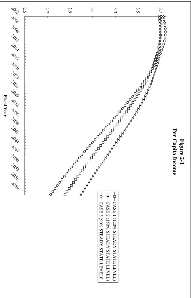
5.1 On Income and Interest Rates: Figure 2-1, and 2-2
As shown in Figure 2-1, per capita income declines after the late 2010’s in all cases. This is because technological progress is assumed to be zero and the forecasted labor supply decreases. The assumption of zero technical progress will be examined in Section 6-1. A decrease in the labor supply comes not only from an aging population but also from a decrease in the total population estimated by the National Institute of Population and Social Security Research in 2002. A surprising result is that after the peak of an aging population, income in Case 2, where the government debt-GDP ratio (the D-G ratio) converges to the highest level, is the highest in all cases. Since in Case 2 the level of outstanding government debts in a steady state is the highest, the resource for private capital is expected to be the lowest, and this result is not intuitive. However, this result can be interpreted as follows: As it will be discussed in Section 5-3, the consumption tax rate in Case 2 is the highest due to interest payments incurred from outstanding government debts, and thus the tax burden ratio in Case 2 is also the highest. Since a consumption tax is imposed on consumption even when an individual becomes old, an increase in the consumption tax rate stimulates savings. This aspect of an increase in the consumption tax rate induces an increase in the supply in the capital market, and results in higher accumulation of private capital. In Case 2, this positive e¤ect is large enough to o¤set a negative e¤ect of the large scale of future outstanding government debts.
The future path of the interest rate determines the future level of marginal pro-ductivity of private capital, and the stock level of private capital. The path also
determines the interest payment of the government, and a magnitude of intertem-poral substitution of consumption. Figure 2-2 shows future interest rates in three di¤erent scenarios. As shown in Figure 2-2, the lowest (the highest) interest rate in a steady state can be achieved when the government de…cits are the lowest (the highest). In Case 3 ( the 90 % D-G ratio), the interest rate converges to 2.15 % in a steady state, and in Case 2 ( the 150 % D-G ratio) it converges to 2.44 %. This implies that the higher are the outstanding government debts the less the private capital stock is. When the amount of the outstanding government debts are higher, public investment, thus the amount of the productive public capital stock, is also higher. An increase in government de…cits reduces the ratio of the private capital stock to the total capital stock, and this implies that private capital is more crowd out when the outstanding government debts are higher.
Furthermore, it is not straightforward to conclude that keeping public investment at a higher level followed by higher outstanding government debts is always preferable, since higher consumption tax rates have to be followed in order to …nance the interest payment incurred by the higher amount of outstanding government debts. If the consumption tax rate is too high to cancel out the positive e¤ect of the high debt policy to increase income, then disposable income would not be higher when the outstanding government debts are higher. Thus, the de…cit policy should be evaluated by the comparison in lifetime utility of di¤erent generations.
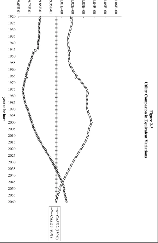
5.2 On Lifetime Utility: Figure 2-3
Although the policy to keep higher government de…cits in the future achieves higher income, the policy should intertemporally be evaluated based on lifetime utility of di¤erent generations. In this paper, all of the cases have been evaluated by comparing their respective levels of utility. Setting di¤erent generations as I and the index measuring the utility level as EV , the de…nition of the utility level index of each generation is given by
EV (I) = ¹ (p
0; p1; y1)
where ¹ (¢) represents the money metric indirect utility function which is de…ned as
¹³p0; p1; y1´´ e³p0; v³p1; y1´´;
where e (¢) and v (¢) denote the expenditure function and the indirect utility func-tion, respectively. p and y denote a price vector and income, respectively, and the superscripts 0 and 1 imply the circumstances under a benchmark policy and those under each proposed policy, respectively. A benchmark case is Case 1 in this paper.
Thus, p0 and y0 are the price vector and income which each generation faces in Case
1. The price vector p0 consists of the interest rate, the wage rate, and tax rates in
Case 1. Thus, if EV (I) is greater (smaller) than 1, it implies that a proposed policy is preferable (not preferable) by generation I to a benchmark policy. Note that a benchmark policy is to maintain a 120 % level of the D-G ratio in a steady sate. Note also that EV (I) measures the evaluation of di¤erent policies by each generation, but
not the evaluation of a policy by di¤erent generations12.
Figure 2-3 shows utility of each generation in Case 2 and Case 3 in comparison with Case 1. Since EV (I) is measured in comparison with Case 1, EV (I) is always unity in all generations in Case 1. Note that the horizontal axis is measured in the year when each generation was born. Compared to a 120 % level of the D-G ratio in a steady state, a 90 % level of the D-G ratio is preferred by almost all generations
12Suppose that in Case 2
EV2(I1) = 1:1;
EV2(I2) = 1:3;
and in Case 3
EV3(I1) = 1:2;
EV3(I2) = 1:5;
are given to generation I1and I2, respectively. This implies that both generation I1 and I2 prefer
Case 2 and Case 3 to Case 1, and both generations relatively prefer Case 3 to Case 2. However, it
except far future generations, but a 150 % level of the D-G ratio is not preferred by any generations born before year 2036. The magnitude of this disadvantage of a debt policy to maintain a 150 % level of the debt-GDP ratio becomes stronger speci…cally among the generations born after the late 1950’s. As has been pointed out in the previous sections, a debt policy to maintain the highest level (150 %) of the debt-GDP ratio achieves the highest income, and the policy have to be followed by the highest successive consumption tax rate in the future. This implies that a debt policy with the highest debt-GDP ratio achieves the highest pre-taxed income, but the lowest post-taxed income. Thus, compared in lifetime utility, this policy is not preferred by the generations of which disposable income is smaller than that in Case 1.
Note also that a debt policy to maintain a 150 % level of the debt-GDP ratio is more preferable to a debt policy with a 120 % level of the debt-GDP ratio by the generations born after 2036. This can be interpreted as follows: As shown in Figure 2-1, per capita income with a 150 % level of the debt-GDP ratio is greater than that with a 120 % level, and the more time passes, the greater becomes the di¤erence in per capita income. This is because a higher consumption tax rate stimulates savings, thus resulting in more private capital accumulation. This increase in private capital accumulation induces an increase in income of future generations. Among the generations born after 2036, this positive e¤ect o¤sets the negative e¤ect of increasing a consumption tax rate to …nance interest payments incurred, and the amount of post taxed income in lifetime with a 150 % level of the debt-GDP ratio is greater than that with a 120 % level. As shown in Figure 2-1, the positive e¤ect of increasing the consumption tax rate to stimulate savings is the smallest in Case 3 with a 90 % level of the debt-GDP ratio in the future, and the more time passes, the greater the di¤erence in the positive e¤ect between a debt policy with a 120 % level (Case 1) and that with a 90 % level (Case 3). Thus, the more time passes, the weaker the magnitude of the advantage of a debt policy to maintain a low level of the debt-GDP ratio in the future.
Case 3, which corresponds to a debt policy to cut the amount of public investment in relatively earlier periods in order to decrease burdens on future generations caused
by higher government de…cits, is preferred by almost all generations when all cases are compared in lifetime utility.
5.3 On the Consumption Tax Rates and Tax Burdens: Table
7 & 8
As has been pointed out in the previous section, maintaining a high level of govern-ment de…cits in the future must be followed by a successive high consumption tax rate due to interest payments incurred from outstanding government debts. Furthermore, a consumption tax rate must increase when government de…cits are reduced. Thus, the intertemporal path of a consumption tax rate depends on the intertemporal pat-tern of government de…cits, and tax burdens on a particular generation also depends on the future government de…cit policy.
Table 7 shows the future consumption tax rate in each case. In relatively earlier periods, the consumption tax rate in Case 3 with a 90% ratio of outstanding govern-ment debts to GDP is higher than those in other two cases. This is because in Case 3 a rapid decrease in the level of outstanding government debts in relatively earlier periods is followed by a high increase in the consumption tax rate. The consumption tax rate increases up to 18.57 % at a peak in year 2008. However, Case 3 achieves the lowest consumption tax rate in the future, since interest payments incurred from the relatively small amount of outstanding government debts are small in the future. On the other hand, in Case 2 a quite high consumption tax rate has to be maintained in the future to …nance interest payments incurred from the huge amount of outstanding government debts. At a peak in year 2050, the consumption tax rate will have to increase up to 20.15 %. The values in detail are given in Table 7.
In Table 8, the tax burden ratio in each scenario is shown. The tax burden ratio is de…ned as the ratio of the total amount of taxes to GDP. As shown in Table 8, since year 2017, the tax burden ratio in Case 3 will be the lowest in all cases. In case 2, where the highest level of outstanding government debts is maintained at a 150% level, the tax burden ratio will increase up to a 37.85 % level. The detailed values are given in Table 8.
5.4 The Contribution Rates ¿
pto the Public Pension Scheme,
Social Security Burden Ratios, and Generational
Ac-counting: Figure 2-4, Table 9 & Figure 2-5
Aso (1997 and 1998) pointed out that intergenerational redistribution in Japan would be caused mainly by an aging population through the existing pay-as-you-go public pension scheme and also that government de…cits would not a¤ect the distribution
among di¤erent generations. Figure 2-4 shows future contribution rates ¿punder the
assumption that the existing scheme is not changed. As shown in Figure 2-4, there is no much di¤erence in the rate in each case, and this paper supports Aso (1997 and 1998). In this simulation, contribution rates rapidly increase until a peak of an aging population in the late 2030’s up to between a 27 % and a 29 % levels in all cases. After the peak of an aging population, the contribution rate increases up to 30.2 % in Case 2 (150 % D-G ratio), and 32.3% in Case 3 (90 % D-G ratio). This di¤erence in the contribution rate among scenarios comes from the di¤erence in income as shown in Figure 2-1.
Re‡ecting increases in the contribution rate in all cases, the social security burden ratio also increases. The social security burden ratio is de…ned as the ratio of the total amount of contribution to the scheme to GDP. Table 9 shows the future ratios. The social security burden ratio converges to a 20.8 % level in a steady state in Case 1, a 19.7 % level in Case 2, and a 22.2 % level in Case 3, respectively. The detailed ratios are given in Table 9.
The concept of the generational accounting originated by Auerbach et al (1998) is also important to discuss intergenerational redistribution through a public pension
scheme13. Hatta and Oguchi (1999) recently estimated the huge amount of transfer
from future generations to old generations through the existing pay-as-you-go public pension scheme, and they asserted that the public pension scheme should be switched to a fully-funded scheme. Figure 2-5 shows the estimated generational accounting based on the model presented in Section 4. Note that the horizontal axis is measured
in the year when each generation was born. Note also that the generational accounting in this paper is de…ned as the net value (the total bene…ts minus the total contribution in lifetime) under the assumption that the contribution is only changed to maintain the existing public pension scheme. As shown in Figure 2-5, the huge amount of transfers is given to old generations from future generations through the existing public pension scheme, and the more time passes the worse the situation. It is forecasted in this simulation that all generations born after 1947 will be worse o¤ in all scenarios.
6 Some Other Results
6.1 The E¤ect of Technological Progress
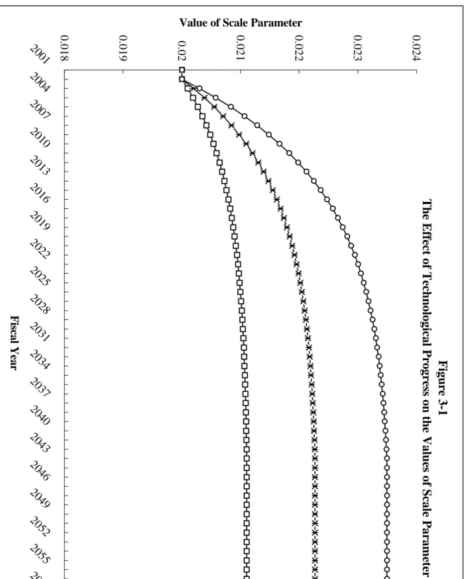
It has been assumed so far that there is no technological progress. This is because results in the simulation heavily depend on the degree of technological progress. How-ever, it is also true that Japan has grown with technological progress. In this section, it is explored how much the results obtained in the previous sections are changed by an introduction of technological progress. In order to highlight the e¤ect of techno-logical progress, a debt policy in benchmark (Case 1) is only examined depending on the di¤erence in the degree of technological progress.
It has been assumed in the following simulation that technological progress starts in year 2003 for 40 years with a diminishing increase in technological progress from a certain level: a 0.5% increase in technological progress per year, a 1.0% increase, and a 1.5 % increase. In these three cases, even though a starting point in the growth rate of technological progress is di¤erent in each case, technological progress ends in year 2043 in all cases, and thus the growth rate of technological progress is zero after year 2043. Under this assumption, technological progress is assumed to be incorporated into the model by changing the scale parameter ª (t), shown in Figure 3-1.
6.1.1 On Income
Figure 3-2 shows the e¤ect of technological progress on per capita income measured in a relative increase with non-technological progress. The vertical axis measures a relative increase in percentage. An introduction of 0.5 % diminishing growth of tech-nological progress for 40 years eventuates in a 8.4 % increase in per capita income in a steady state, and 1.0 % diminishing growth achieves a 18.3 % increase in per capita income. In the case of 1.5 % diminishing growth of technological progress generates a 30 % increase in per capita income compared to non-technological progress. 6.1.2 On Lifetime Utility
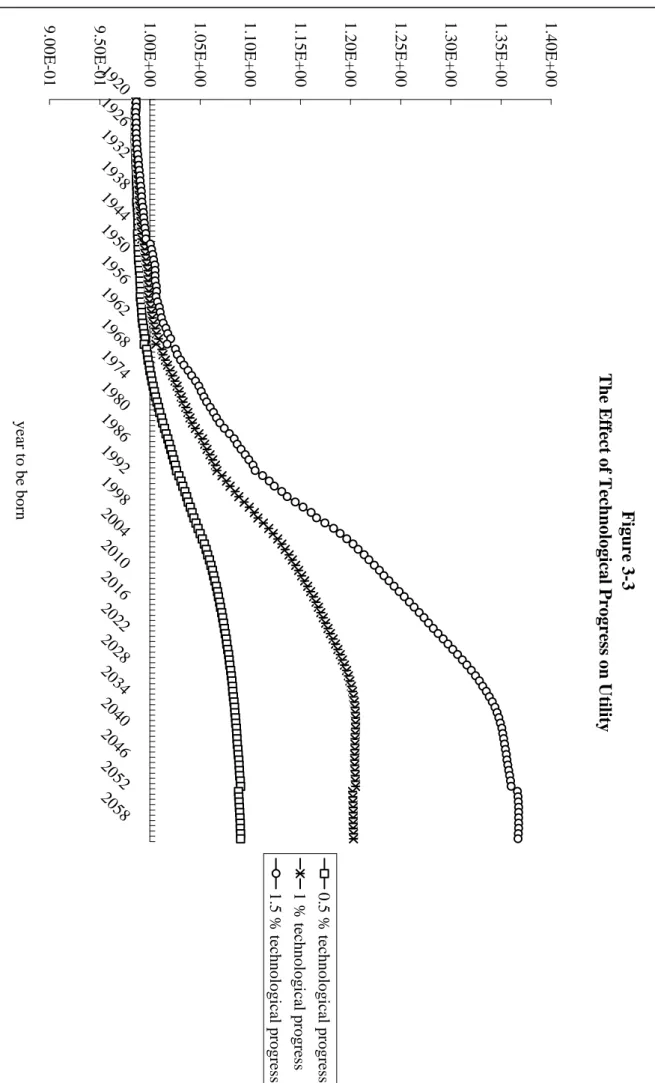
Figure 3-3 shows the e¤ect of technological progress on lifetime utility measured in equivalent variations in comparison with the no-technological progress case. Thus, if the value of a generation is greater (smaller) than unity, then technological progress more (less) preferable by the generation.
As time passes, generations get better o¤ due to technological progress. As shown in Figure 3-2, this is because income with more technological progress is higher, and an increase in income is larger as time passes.
There is another result that technological progress is not preferable by old genera-tions, which is not intuitive, since technological progress should have a positive e¤ect on all generations. This result can be interpreted as follows: The future income level with more technological progress is relatively higher than that with no-technological progress.. This implies that households who want to have smooth consumption in their lifetime save less when they can expect to have more technological progress. A decrease in savings reduces supply in the capital market, and the resources for pro-duction in the private sector decrease. Thus, technological progress partly operates to reduce income through the optimal behavior of households when households expect higher income due to technological progress. If this e¤ect of technological progress to reduce savings is stronger than a positive e¤ect on production to induce higher income, then it is possible to decrease lifetime utility. Since the positive e¤ect on production is accumulated through time, the negative e¤ect of technological progress
on income through the capital market relatively becomes smaller as time passes. 6.1.3 On the Consumption Tax Rate
Table 10 shows the e¤ect of technological progress on the consumption tax rate in the future. A 0 % increase in growth of technological progress corresponds to Case 1 in Section 5-3. In Case 1, a peak in the consumption tax rate is obtained in year 2018. At the peak, the consumption tax rate has to increase up to 16.3 % in 0 % technological progress. However, it increases up to 14.8 % in 0.5 % technological progress, 13.2 % in 1.0 % technological progress, and 11.6 % in 1.5 % technological progress, respectively. As shown in Table 10, the degree of an introduction of technological progress does matter when the amount of burdens on future generations is explored.
6.2 The E¤ect of E¢ciency in Public Investment.
It has been argued in Japan that an expansion of public investment does not stimulate the Japanese economy e¢ciently in the short-run due to a decrease in the multiplier e¤ect. As pointed out by Ihori and Kondo (1998), there is another role of public investment to a¤ect the supply side in the long-run, and they argued that e¢cient public investment is crucial for stable economic growth in the long-run. If not only the short-run e¤ect but also the long-run e¤ect weaken, keeping a certain level of public investment in the future only leaves the huge amount of burdens on future generations. In this section, the e¤ect of ine¢ciency in public investment in the fu-ture is explored by assuming that a certain amount of public investment does not contribute to production in the private sector, even though the future level of public investment does not change. In this paper, the e¤ect of ine¢ciency in public invest-ment is examined by changing the value of ¯, the elasticity of the stock of productive public capital with respect to the private production function. By setting ¯ = 0:248; 0:124, and 0 in Case 1, the e¤ect has been examined. ¯ = 0:248; which is the latest value of ¯ estimated by Yoshino and Nakajima (1999), corresponds to a fully e¢cient case in public investment (a 0 % ine¢cient case). ¯ = 0:186, ¯ = 0:124 and ¯ = 0 correspond to a 75 % e¢cient case (a 25 % ine¢cient case), a half e¢cient case ( a 50
% ine¢cient case), and a zero e¢cient case (a 100 % ine¢cient case), respectively14. It has also been assumed that until year 2002 public investment is fully e¢cient, and ine¢ciency in public investment occurs in year 2003. The ine¢ciency is assumed to persist after 2003. The following results have been obtained in Case 1.
6.2.1 On Production (Income)
Figure 4-1 shows the e¤ect of ine¢ciency in public investment on income in compar-ison with a full e¢cient case (¯ = 0:248), under the assumption that the amount of public investment is the same in all cases. In a steady state, when there is 25 % ine¢ciency ( a 75 % e¢cient case) in public investment, a 6.5 % decrease in income is induced. 50 % ine¢ciency in public investment results in about 15 % decrease in income in a steady state, and income in a steady state decreases at 30 % if public investment does not contribute to production in the private sector at all.
6.2.2 On the Consumption Tax Rate
Ine¢ciency in public investment also a¤ects the future consumption tax rate. Table 11 shows how much the consumption tax rate is a¤ected by ine¢ciency in public investment. The more time passes, the greater becomes the negative e¤ect of inef-…ciency in public investment on the consumption tax rate. In a steady state, the consumption tax rate increases at about 1.95 % when there is 25 % ine¢ciency in public investment, and at 4.98 % when there is 50 % ine¢ciency. If public investment does not contribute to the private sector production, then the consumption tax rate becomes over 26 %, and there is 11.66 % di¤erence in the consumption tax rate in a steady state between a full e¢cient case and a zero e¢cient case.
6.2.3 On Lifetime Utility
Figure 4-2 shows the e¤ect of ine¢ciency in public investment on utility measured in equivalent variations in comparison with a full e¢cient case. Thus, if the value of
14Although the production function is di¤erent in this paper, a zero e¢cient case corresponds to
a generation is greater (smaller) than unity, then ine¢ciency in public investment is more (less) preferable by the generation.
As time passes, generations get worse o¤ due to ine¢ciency in public investment, and the number of future generations which are worse o¤ increases as the degree of ine¢ciency increases. When there is 25 % ine¢ciency, all generations born after year 1977 are worse o¤, and when there is 100 % ine¢ciency in public investment gener-ations born after 1973 are worse o¤. The more ine¢ciency increases, the greater is the e¤ect of ine¢ciency on utility of all generations. Since the cost paid by house-holds through taxation to maintain a certain level of public investment does not change, greater ine¢ciency in public investment gives future generations more bur-dens through the negative e¤ect on the accumulation of pubic capital.
Furthermore, ine¢ciency is more preferable by old generations. This result is not intuitive, since ine¢ciency should have a negative e¤ect on all generations. However, this result can be interpreted as follows. Ine¢ciency in public investment reduces income in the future. This reduction in the future income is not desirable for house-holds who want to have smooth consumption in their lifetime, and they save more when they are relatively young in order to have smooth consumption. Their response is greater as the expected reduction in their income is greater. An increase in sav-ings induces a shift of supply in the capital market, and the resources for production in the private sector increase. Thus, ine¢ciency operates to induce higher income when households expect the reduction of their income. If this positive e¤ect of inef-…ciency to stimulate savings o¤sets the negative e¤ect to reduce public capital, then ine¢ciency increases lifetime income. Since the latter negative e¤ect is accumulated through time, it is more likely for old generations to prefer ine¢ciency in public investment.
7 Concluding Remarks
This paper has tries to examine the e¤ects of government de…cits, public capital and the public pension policy on the tax burden, capital accumulation and economic
welfare in the transition to an aging Japan by applying a simulated method in the expanded life cycle general equilibrium growth model. This paper expanded Kato (2000, 2002b) by incorporating public capital into the model and re-examined the e¤ects of the future Japanese government debt policy by presenting several scenarios. The results obtained in this paper are summarised as follows: First of all, a cut in future public investment associated with a decrease in government de…cits reduces income and production in the future. A future decrease in government de…cits avoids an increase in a consumption tax to …nance interest payments incurred from the huge amount of outstanding government debts in the future, but at the same time a rel-atively small increase in a consumption tax weaken a positive e¤ect of consumption taxation to stimulate savings, thus resulting in production being smaller in the sce-nario to reduce future government de…cits. However, if such a policy is evaluated in lifetime utility of all generations, then it is most preferable by all generations, because such a policy achieves the highest disposable income. Thus, even though a policy to reduce future government de…cits have to be followed by the reduction in pubic investment, the government should reduce the government de…cits.
Secondly, as pointed out by Aso (1997 and 1998), and Hatta and Oguchi (1999), intergenerational redistribution through the existing pay-as-you-go public pension scheme can be explained by an aging population in Japan. The critical generation which is worse o¤ through the existing public pension scheme is nearly the same as that pointed out by Hatta and Oguchi (1999).
Thirdly, the degree of technological progress does matter for the analysis. An introduction of 0.5 % diminishing growth of technological progress for 40 years even-tuates in a 8.5 % increase in per capita income in a steady state, and 1.0 % diminishing growth achieves a 18.2 % increase in per capita income. In the case of 1.5 % diminish-ing growth of technological progress generates a 30 % increase in per capita income compared to non-technological progress. The di¤erence in technological progress af-fects all important policy variables such as tax rates and the burden ratio.
Finally, as time passes, generations get worse o¤ due to ine¢ciency in public investment, and the number of future generations which are worse o¤ increases as the
degree of ine¢ciency increases. Ine¢ciency also reduces future income. In a steady state, when there is 25 % ine¢ciency in public investment a 6.5 % decrease in income is induced. 50 % ine¢ciency in public investment results in about 15 % decrease in income in a steady state, and income in a steady state decreases at 30 % if public investment does not contribute to production in the private sector at all.
Several results have been obtained in this paper, and the following points are es-pecially important as policy implications: Higher economic growth is necessarily not more desirable, and only targeting high economic growth would mislead us as to the economic policy. The economic policy should be evaluated based on lifetime utility of di¤erent generations, and one of the current policy options that the government should reduce the public investment level in the future in order to decrease govern-ment de…cits is most evaluated by all generations even though it would be politically di¢cult. Furthermore, when the government policy in Japan is evaluated in terms of intergenerational redistribution, it should also be compared in welfare. As has been pointed out, it seems that the existing pay-as-you-go public pension scheme in Japan is not actuarially fair, and thus there is signi…cant distortion in generational accounting in terms of intergenerational transfer. Although the distortion through the scheme, which causes the huge amount of transfer from future generations to old generations, should obviously be eliminated, the fact that public capital in Japan has been accumulated by public investment in the past partly …nanced by taxes imposed on old generations should also be taken into account. The huge amount of outstand-ing government debts mainly caused by public investment is the result of the past Japanese government policy, and it is just a policy to postpone the …nancial burden. Thus, if the Japanese government policy is evaluated in terms of intergenerational redistribution, these complicated aspects should all be taken into account. This can only be possible by the consideration within a general equilibrium framework, which this paper has been based on under the assumption that the existing public pen-sion scheme is maintained in the future. The result in this paper that an economic policy to cut the future public investment in order to reduce government de…cits is most preferable even by future generations would give another interpretation of the
Appendix
For the utility maximization problem over time, the Lagrange function is given such that: L = U + 80 X s=1 ¸s 8 > > > > > < > > > > > : As+1¡ 0 B B B B B @ [1 + (1 ¡ ¿r(t)) r (t)] As + (1 ¡ ¿y(t) ¡ ¿p(t)) w (t) es+ bs +as¡ (1 + ¿c(t)) Cs 1 C C C C C A 9 > > > > > = > > > > > ; + 80 X s=1fÁ2s (DYs¡ Cs) + Á1s(Cs¡ CMIN)g ;
and the …rst order conditions are
Ss(1 + ±)¡(s¡1)C ¡1 ° s ¡ ¸sP C (t) ¡ Á2s+ Á1s = 0; ¡¸s+ ¸s+1ARA (t) = 0; Á2s(DYs¡ Cs) = 0; Á1s(Cs¡ CMIN) = 0; where P C (t) = 1 + ¿c(t) ; ARA (t) = 1 + (1 ¡ ¿r(t)) r (t) ;
and ¸s, Á1s and Á2sdenote the Lagrange multipliers for (2), (3) and (4), respectively.
The above …rst order conditions yield
Cs = µ ANCs£ C ¡1 ° 1 + AOBs ¶¡° ; where ANCs = ANB (t) S1(1 + ±)(s¡1) Ss ; ANB (t) = P C (t) P C (1)Q80 t=1ARA (t) ; P C (t) = 1 + ¿c(t) ; ARA (t) = 1 + (1 ¡ ¿r(t)) r (t) ;
and AOBs = (1 + ±)(s¡1) Ss 8 > > > > > < > > > > > : ANB (t) 2 6 4 Á11¡ Á21¡ P C (1)P80 s=2Á2sDYs³Qst=1¡1ARA (t) ´ 3 7 5 +Á2s¡ Á1s 9 > > > > > = > > > > > ; :
From (5), the optimal consumption behaviour of all ages can be derived if the
initial consumption C1 is speci…ed, and the savings level can be calculated from (2)
and (5). To derive C1, (5) is substituted into the life cycle budget constraint such
that X P C (t) Cs Q ARA (t) = X(1 ¡ ¿y(t) ¡ ¿p(t)) w (t) es Q ARA (t) +XQ bs ARA (t) + X as Q ARA (t):