Asymptotic Theory of Selection by Relative Rank with Low Cost

Journal of the Operations Research Society of Japan

Vo!. 36, No. 3, September 1993

ASYMPTOTIC THEORY OF SEI,ECTION BY RELATIVE RANK WITH LOW COST

Sigeiti Moriguti

Professor Emeritus. University of Tokyo

(Received September 14, 1992; Revised January 6, 1993)

Abstract Selection from among n objects by relative rank with no recall - the "secretary problem" - in the asymptotic case when n --+ 00 is considered, assuming that k, the cost ratio, is O(l/n), i.e. K = k· n is a finite constant. Starting from the special case of K = 0, the situation changes smoothly as K grows and eventually approaches the "medium cost'> case. Thus, the ratio of expected cost of observation to the expected rank goes smoothly from 0 to 1 as K goes from 0 to 00.

1. Introduction

The "classical secretary problem" (cf. Chow et a1. (1964)) assumes that the cost of observation i8 O. This might be considered to be too optimistic in many practical cases, especially when n, the total number of object;.;, is very large. So Moriguti (1993a) discussed the ba8ic theory of the "secretary problem" with cost. Subsequently, Moriguti (1993b) dealt with asymptotic behavior with "medium cost'·. There the cost ratio:

(1.1 ) k = cost of observing one object

loss of getting one lower expected rank was kept to be a finite constant while n -+ oc

It turns out that there is a considerable gap between the "classical" case of k == 0 and the "medium cost" case of k = 0(1). To bridge the gap, we discuss in this paper the "low cost" case, assuming that

(1.2) K= k·n

is kept constant when n -+ 00.

The "classical" (no cost) case is also included, as a special case, in this paper. In fact, the results of that case are found to be useful for numerical computations in the non-zero

"low cost" case.

As in the previous paper on the "medium cost" case (Moriguti (1993b)), not only the expected value of the attained absolute rank r, but also the distribution of r is also given here. The latter result is perhaps new even in the "classical" case.

2. Notations and fundamental formulae.

Let us introduce the following notations:

(2.1) u. =

i/n,

(2.2) T(u) = tj, (2.3) C(u) = Cj,

(2.4) E(u)

=

e;jn, (2.5) Us

=

isln, (2.6) Q(u)

=

Q(i).

Then, as n -t 00 with s finite, we get

(2.7)

from (2.15) of Moriguti (1993a). Q(u) is continuous at u = us+l, as easily proved. This is the probability that no stopping occurs at i = un or before.

The expected number of observations until stopping is given by nE(O), where (2.8)

from (3.4) of Moriguti (l993a).

The expected rank of the selected object is given, from (5.4) of Moriguti (19~13a) and (2.7) above, by

(2.9)

The recurrence formula for the conditional total loss tj, (6.7) of Moriguti (1993a), be-comes now the differential equat ion

(2.10) _ dT{u)

=

~(.s

+

₂ 1)

+ [." _

H ~T(u) (Us

:s:

u :S:Us+I)·

du 2u u

(Note (1.2) above.) Using the integration factor 1/us, it can be transformed into (2.11)

which gives (2.12)

for s

?:

2, and

(2.13) --T(1.1) 1 == - - 2 1 "

+

h loge u

+

Al (UI:S: u:S: U2)

Secretary Problem with Low Cost 177

for s

=

1, where AI, A2, A3,'" are constant each in the corresponding interval.

The equation (6.8) of Moriguti (1993a) which gives the optimum criterion now becomes (2.14) s = 1l.5T(us ) (0' = 1,2,···)

in the limit as n -, 00. Using (2.14) together with (2.13) and (2.12), we get

(2.15)

:r -

:~

₌

~

(:r -

:~)

₊

_{I\ loge}

~:

_{(s = 1).} (2.16) _us s+1

S(

1 1)

I\

(1

1)

5+1 -- us+1

=

2'

u5+1 - us+1

+

S - 1 u5- 1 - u5-1

8 s+l 5 8+1 5 5+1

(8 ~ 2). Now, let us rewrite (2.12) in the form

(2.17) whence (2.18)

(2.19)

8 I\u

T(u.) = -

+ - - -

A5us (us:S

u:S

U5+1, 8 ~ 2),

2u 8-1 I S I\ 1 ) T (U)

=

- - 2

+ - - -

A5sU 5 -- (Us:S U

:S

U5+1,

s

~ 2 , 2u 8-1 " S ')

T (u)

=

3' - A5S(S - l)uS-~ (us:S u

:S

U5+1, 8 ~ 2).

u Also, (2.13) gives us (2.20) (2.21) (2.22) T"(u) ___ 1 _ I\ ( U1 :S u :S U2 . ) u3 _U

These formulae will be used in Appendix 2.

So far. the derived formulae are almost exactly the same as those in Section 2 of Moriguti (1993b). But from here on, we shall see more or less different pictures.

3. Case of no cost.

Now let us consider the case where k = O. namely the so-called "classical secretary problem" .

W-ithout the term containing I\, the formula (2.15) becomes the same as (2.16) with

.5 = 1, and (2.16) can now be transformed into

(3.1 ) S u~+l S +~' U8+1' 5+1 (S ~ 1),

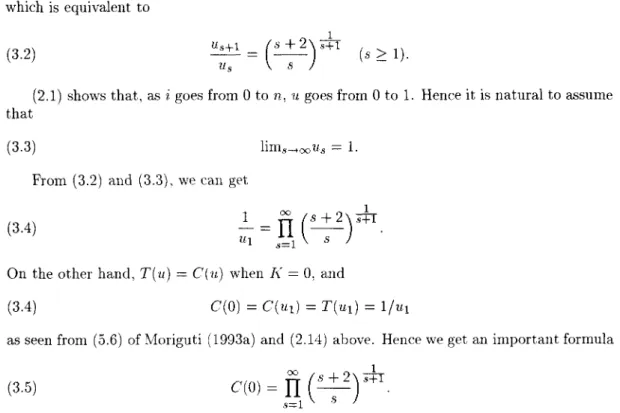
which is equivalent to

(3.2)

1

Us+l =

(8

+

2)

S+I

(82:

1).

Us s

(2.1) shows that, as i goes from 0 to n, 11 goes from 0 to 1. Hence it is natural to assume

that (3.3)

From (3.2) and (3.3), we can get

(3.4)

1

~=fi(S+2)s.n.

Ul s=1 S On the other hand, T(u) = C(Il) when J{ = 0, and

(3.4) C(O) = C(Ul) = T(utJ = l/Ul

as seen from (5.6) of Moriguti (1993a) and (2.14) above. Hence we get an important formula

(3.5) C(O) = fi

C

+ 2)

sir.

8=1 s

The infinite product on the right-hand side is convergent and has the value 3.869~12 (for the details, see Appendix 1).

Starting with Ul = l/C(O) = 0.25843, we can get the values of U2,U3,' .. using (3.2) successively. The first 100 values are listed in Table 1.

Table 1. First 100 values of U8 for J{ = O.

8 U(8) 8 11(8) 8 U(8) 8 U(8) 8 U(8)

1 .2584 21 .!H12 41 .9529 61 .9680 81 .9758 2 .4476 22 .!H49 42 .9540 62 .9685 82 .9760 3 .5640 23 .!H84 43 .9551 63 .9690 83 . 976~; 4 .6408 24 . !3216 44 .9561 64 .9695 84 .9766 5 .6949 25 .9246 45 .9570 65 .9699 85 .9769 6 .7350 26 .!3273 46 .9579 66 .9704 86 .9771 7 .7658 27 .!3299 47 .9588 67 .9708 87 .9774 8 .7903 28 .13322 48 .9596 68 .9712 88 .9777 9 .8101 29 .13344 49 .9604 69 .9716 89 .9779 10 .8265 30 .9365 50 .9612 70 .9720 90 .9781 11 .8403 31 . !3385 51 .9619 71 .9724 91 .9784 12 .8521 32 .9403 52 .9626 72 .9728 92 .9786 13 .8623 33 .13420 53 .9633 73 .9732 93 .9788 14 .8711 34 .9437 54 .9640 74 .9735 94 .9791 15 .8789 35 .9452 55 .9646 75 .9739 95 .9793 16 .8858 36 .9467 56 .9652 76 .9742 96 .9795 17 .8920 37 .9481 57 .9658 77 .9745 97 .9797 18 .8975 38 .B494 58 .9664 78 .9748 98 .9799 19 .9025 39 .B506 59 .9669 79 .9752 99 .9801 20 .9070 40 .B518 60 .9675 80 .9755 100 .9803

Secretary Problem with Low Cost ₁₇₉

The cumulative distribution fUIlction of the number of observations is 1 -

Q(

u), where

Q(u) is given by (2.7) above.

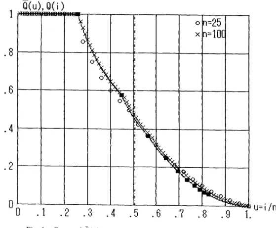
The curve of lj ( u) vs. u is shown in Fig. 1, together with points showing Q (i) vs. i / n for some finite values of n. (The latter points were obtained using (2.5) of Moriguti (19H3a).)

The dot-dash vertical line corresponds to the expected number of observations (divided by n):

(3.6)

which is given by (2.8) above.

1

Q(u),Q(i)

£(0) = 0.50647

o

n=25

X

n=10[

Fig. 1. Curve of Q(11) for K = 0 with points for n

=

25 and 100. 4. Distribution of the absolute rank.

The basic formulae for the probability dis;ribution of the absolute rank T of the selected

object was developed in Section 4 of ~lorigllti (1993a). The corresponding asymptotic for-mulae for low-cost cases are to be developed here. Since they are applicable to both zero-cost and non-zero-cost cases. we change the SediGn. But since actual numerical values will be given in this Section only for the zero-cost case, the reader may take this Section as the continuation of Section 3, for the tinlE' being.

The distribution of r is a discrete one. In particular, the probability that T = 1 is derived

from (4.13) of l\loriguti (1993a) as

and for the no-cost case, its numerical value is

(4.2) f(l) = 0.50647 - 0.25843 = 0.24804.

For a general value of r, its probability is given by (4.11) of Moriguti (1993a), and f(i, r)

there is different from f(i, 1) only for such i that 8;

<

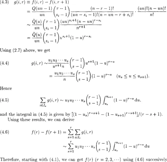
r (compare (4.12) and (4.14) there). For such i, (4.15) there approaches, as n --t 00,

(4.3) g(i, r)

==

f(i, r) - f(i, r

+

1)

= Q(un -

1)

(r --

1)

(n -

r

-1)! . (un)!(n - un)!

un Si .-1 (un - 8; - 1)!(n - l1n - r

+

Si)! n!

rv Q(u)

(r

-1)~Un)Si+1(n -

unt-

si

un Si - 1 nr₊₁

= Q(u)

(r -

1 )VSi+l(1 _ ur-Si

un Si - 1

Using (2.7) above, we get

( 4.4) g

(. ) u

l r r v - - - - -1

uz ... u

s

(r-1)

U s+l( 1 - u )r-s , us+1_{n S - 1} = U1 U2" 'Us

(r

-1) (1 _

_ur-s n 8-1 Hence (4.5) ₍r -

1)

l

u '+l

L

g(i, r) ~, Uj U2" . Us (1 - ur-s du,

iEI, S - 1 u,

and the integral in (4.5) is given by [(1 - us)'"-s+l - (1 - Us+l)'"-s+lj/(r - S

+

1).

Using these results, we can derive

r

( 4.6) f(r) - f(r+ 1) =

L

Lg(i,r) s=1 if I,

Therefore, starting with (4.1), we can get

f

(r) (r = 2,3" .. ) using (4.6) succesively. After that, the c. d. f. F(r) can be obtained by cumulative summation of f(r).

Table 2 lists

f

(r) and F (r) for r = 1, ... , 40 in the zero-cost case.

Fig. 2 shows the graph of F(r) as a broken line, together with the points showing F(r)

for some finite values of n, all in the zero-cost case. The vertical dot-dash line shows the expected value (3.5).

5. Case of non-zero cost.

Now, let us proceed to the case where [{

>

O. For S ;::: 2, from (2.12) we gEt

(5.1)

T..' 2

" n U s+1

uT(u)=--+---Au (us~u~us+l)

Secretary Problem with Low Cost 181

Table 2. Distribution of the rank r of the selected object (K

=

0).

r f(r) F(r) r f(r) F(r) r f(r) F(r) r f(r) F(r) 1 .2480 .2480 11 .0091 .9694

:n

.0007 .9939 31 .0002 .9B74 2 .1991 .4472 12 .0065 .9758 ~~2 .0006 .9945 32 .0002 .9B76 3 .1541 .6012 13 .0047 .9805 23 .0005 .9950 33 .0002 .9B77 4 .1151 .7164 14 .0034 .9839 24 .0004 .9955 34_ .0001 .9B79 5 .0835 .7B98 15 .0026 .9865 25 .0004 .9959 35 .0001 .9B80 6 .0590 .8:;88 16 .0020 .9885 :26 .0003 .9962 36 .0001 .9H81 7 .0409 .8B98 17 .0016 .9901 27 .0003 .9965 37 .0001 .9982 8 .0281 .9279 18 .0013 .9914 :28 .0003 .9968 38 .0001 .9983 9 .0192 .9471 19 .0010 .9924 :29 .0002 .9970 39 .0001 .9984 10 .0132 .9G02 20 .0008 .9932 30 .0002 .9972 40 .0001 .9H85

F(r)

1

~

...

.-.. i

~

~

,

,

,

~/

i'

(:

o

n=25

X

n=100

i

,

,

,

I

fl

I I I 1 _Lt;1 1 I L1 1 1 1 I 1 1 1 1 I 1 1 I 1 1 1 I 1 1 1 1 1 1 1 1

r

.8

. 6

. 4

.2

5

10

15

20

25

30

35

41)

Fig. 2. Curve of F(r) for K = 0 with points for n = 25 and 100. and, from (2.13),

(5.2)

Using (2.14) with (5.1), we have (5.3) 1.'_ 2 s I1 Ii.s A s+1 s =

-+ --- -

u 2 8-1 s s ' whence (5.4) A vs+!

=

Kl{ -::

(s

>_

2). S s s-L 2

Also, using (2.14) replacing 8 with 8

+

1, we have 8 Ku2 s+l = _+~_Aus+l 2 8 - 1 s s+I, (5.5) whence (5.6) A 'us+1 _ KU;+1 _ _{s s+1 - 8 - 1} 8

+

₂ 2 (82:2). From (5.4) and (5.6), we get an instrumental formula

2Ku; - 8(8 - 1) _ 2Ku;+1 - (8 - 1)(8

+

2)

uS

s+1 us_s+1 +1

(5.7) (82:2).

Similarly, we can derive, from (5.2) and (2.14),

1 3 U 2

2}" 2 "ul = 2}' 2 \. u2

+

loge-' Ul (5.8)

Formula (5.7) implies:

Proposition[5a] If 2Ku; = 8(8 -- 1) then 2Ku;+1

=

(8 - 1)(8

+

2), and vice versa; Proposition[5b] If 2Ku;+1

>

(8 - 1)(8

+

2) then 2Ku;

>

8(8 - 1)

>

(8 - 2)(8

+

1); Proposition[5c] If 2Ku;

<

8(8 -- 1) then 2Ku;+1

<

(8 - 1)(8

+

2)

<

8(8

+

1). It can be proved (see Appendix 2) that:

Proposition[5d] The function T(u) has a minimum at one and only point

u

which lies in the interval (ut, 1);

Proposition[5e] If

u

is in the interval [us, Us+l) and 8 2: 2, then

(5.9)

;~~~~;

- 8(8 -1) =

!(~s)S+I,

2li..u2 - 8(8 -1) 8 u

(5.10)

2Ku;~;:

- (8

+

2)(8 -1) = !(US+1)S+I. 2.hu2_{-8(8-1) 8 U}

Proposition[5f] If

u

is in the interval (Ul, u2),then (5.11)

(5.12) 3 1

2 1> Tf 'U'2 2

+

loge U2

=

21.'-2 1> '11,

+

1

+

loge

u.

Proposition[5g] If

u

is in the interval [US" us'

+

1) then

2Ku; 2: 8(8 -1) for 8

=

8*,8* -1", ·,l,and

2K u;

<

8( 8 - 1) for 8

=

8*

+

1,8*

+

2, .... Proposition[5h] The s* defined in [5g] is determined by the formula

Secretary Problem with Low Cost 183

where int[x] denotes the greatest integer not greater than x.

For computational purpose, we may use a temporary variable (5.14)

and the notations 'ii = J(2K) . il, Vs = J(2K) . uses = 1,2," .). Then all the expressions like 2K u2 in the above formulae should be changed into corresponding v2.

Given

v,

we proceed as follows:

Step 1. Determine s* by (5.13), and obtain Vs' and Vs'+1 by (5.9), (5.10) if s* ;::: 2, or by (5.11), (5.12) if s*

=

l.

Step 2. If s*

>

2, then use (5.7) to get the value of Us from U s+l for s

=

s* - 1, s* - 2"",2,

and finally use (5.8) to get U1 from U2. In each step, successive approximation is to be used, using for example

(5.15) Vs

=

Js(s - 1)

+

v:+1[v;;+1 - (s - l)(s

+

2)]/v:ti

for s ;::: 2.

Step 3. Use (5.7) to get the value of U_{s+1 from lIs for s}

=

s*

+

1, s*

+

2,···. In this case,

Newton's method is more efficient than the simple iteration like (5.15). Theoretically, this step could go indefinitely. In practice, however, it is wise to store the value of

V s+1 1 s

+

2

ds = log log -e Vs S

+

1 e s

(5.16)

and stop at such s that

I

ds

I

is sufficiently small. The idea is that the series (5.17) D = d1

+

d2

+ ...

converges much faster than the series (5.18)

and the numerical value of (5.18) can easily be obtained by adding

00 1 8+2

L - -

loge . - = 1.353130

s=1 s

+

1 s

(5.19)

(cf. Appendix 1) to the value of (5.17).

Step 4. Once the value of (5.18) is obtained, it is easy to get (using the value of VI which is already known) ( 5.20) Voo

=

J(2K). Step 5. Compute (5.21) K =: v~/2, values of il ==

v /

J

(2K) and (5.22)

1

u(s)=i(s)/n

. 8

I---

---

r____.

---

-

I----I---

I~

r---I'---

r----

r---...-r---.-

'--r--..

---

_---

f-..

r--...

,--/ ~

r----..

V

I---

t---1---

I---..

~

---

I---

---. 6

.4

.2

5

10

15

20

25

30

35

iJ

---..

r--.-

---...

-

r---40

45

50

s=50

s=20

s-lO

s=5

s=4

s=3

s

2

s=1

K

Fig. 3. Curve., of Us (for some values of s) and u vs. K. Table 3. K for 50 values of v.

v K

v

K

v

K v K v K .1 .0748 1.1 7.1385 2.1 16.2780 3.1 26.7814 4.1 38.5485 .2 .2989 1.2 7.7130 2.2 16.9860 3.2 27.5953 4.2 3B.4608 .3 .6708 1.3 8.0522 2.3 17.4398 3.3 28.1316 4.3 40.0686 .4 1.1874 1.4 8.1717 2.4 17.6488 3.4 28.3977 4.4 40.3813 .5 1.8424 1.5 9.1971 2.5 18.4362 3.5 29.0770 4.5 41.0009 .6 2.6238 1.6 10.4433 2.6 19.9703 3.6 30.8553 4.6 4a.0045 .7 3.5106 1.7 11.7231 2.7 21.5098 3.7 32.6205 4.7 44.9801 .8 4.4677 1.8 13.0010 2.8 23.0158 3.8 34.3299 4.8 46.8815 .9 5.4412 1.9 14.2274 2.9 24.4368 3.9 35.9285 4.9 48.6502 1.0 6.3587 2.0 15.3411 3.0 25.7121 4.0 37.3556 5.0 50.2231

This completes the procedure to get K,ll, and Ul, UZ, ... for given

v.

Fig. 3 shows the values of us(s = 1,2." .. 5; 10, :20, ... ,50) and u plotted against K.

If one wants to know the value of

v

corresponding to a desired value of K, then e.g. a bi-section method can easily be programmed, starting from two values of

v

giving values of K one of which is too small and the other too large. Table 3 will be useful in getting those starting values. For example, we get 7) = 0.85445,1.56486,2.60193,4.28564 for K =

5,10,20,40 respectively.

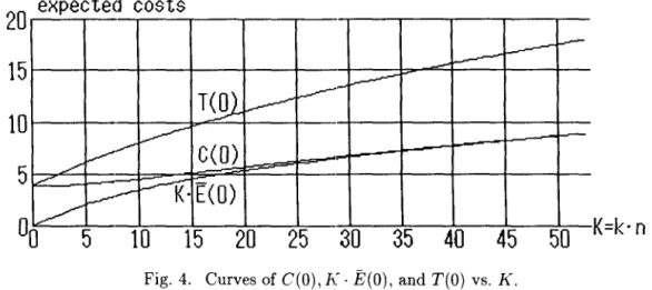
For a given v(or K), using the computed valuesus(s = 1,2,"') and the formulae (2.8), (2.9), it is easy to get the values of expected interview cost K· £(0), expected absolute rank

C(O), and the expected total "loss"

Secretary Problem with Low Cost 185

It can also be computed by the formula (5.24)

and the equality of (5.23) and (5.24) can be used as a check.

Fig. 4 plots computed values of C(O), 1< . E(O), and T(O) against 1<. It is interesting to note the tendency that C(O) and 1< . E(Ol approach each other as 1< becomes larger and larger. This indicates smooth transition to the "medium cost" case treated in Moriguti (1993b).

20

expected costs

5

~

I---

~ ~...-~

T~

~

V--

-l..---

C(O)

L v

Pj{. E(O)

V--~

15

10

5

10

15

20

25

30

35

40

45

50

K=k·n

Fig. 4. Curves of C(O), K· E(O), and T(O) vs. K.

6. Conditional expected costs.

In this Section, let us observe the behavior of the functions C(u), 1< . E(u), and T(u).

These are the expected rank, expected interview cost, and the expected total "loss", respec-tively, under the condition that stopping does not occur at i = un or before.

The recurrer.ce formula (3.6) of Moriguti (1993a) becomes now the differential equation

dE(u) s

-- -- -- = --E(u)

+

1 (us::; u ::; Us+1). du u

(6.1)

Its general solution is

(6.2) E(u)

=

U/(8 - 1)

+

Esu s (us::; u ::; u s+1, s 22),

=

-u ·loge u

+

E₁u (U1::; u ::; U2),

=

-u

+

Eo (0::; 11 ::; U1),

where each constant Es is to be determined successively, starting from E(O) discussed in Section 5.

Fig. 5 shows the result of computation along this line for K = 0,5,10, 20,and 40. As

K increases, the curve comes to resemble the case of "medium cost", especially in the right part of the graph (i. e. as u ~ 1).

The expected rank of the selected object under the condition that stopping does not occur at i

=

un or before is represented by C(u). The recurrence formula (5.6) of Moriguti (1993a) becomes now the differential equation

(6.3) _ dC(u) __ s(s

+

1) _ ~C(u)

E(u)

· 7

*-*IK=O

_{G---£l1! K}

₌₅

~

K=lO

8--£l

K=20

.6

~

K=40

~~

0

.~

(~""

₀

~

~

~"

"

--..

_{"'A ~} .r::r ... ~ ~ -R-~ ~

.5

· 4

· 3

.2

· 1

~ ~

'-

---o

o

. 1

Its general solution is (6.4)

.2

.3

.4

.6

. 7 . 8

Fig. 5. Curves of E(u) for several values of K.

C(u) = ;u - Csus (us:::; u :::; Us+l, S

2':

1),

= Co (0:::; U :::; Ul),

.9

1.

u

where each constant Cs is to be determined successively, starting from C(O) given by (2.9) above.

Fig. 6 shows the result of computation along this line for K = 0,5,10,20, and 40. Here again, we see the resemblance to the "medium cost" case in the right part.

The conditional total "loss"

(6.5) T(u) = C(u)

+

K . E(u)

can be computed from the value; of C( u) and E(u). On the other hand, we can also compute

T(u) starting from (5.24) and utilizing

(6.6) T(u) = T(O) - K· u (0:::; u :::; ud,

(6.7)

and (6.9) (6.10)

C(u)

25

20

15

10

5

_,

Secretary Problem with Low Cost 187

>*---*

K=O

f

e---£)

K=5

~

K=10

~

!3---£1

K=20

J

1s---6

K=40

I

/

V

~ ~ ... ::;;;;.,;.. ~

. 1

.2

. 3

. 4

.6

. 7

.8

. 9

1.

u=: iln

Fig. 6. Curves of C (u) for several values of K.

A

_(KU;

S)

1 s - S _ 1 -

2

us+1 '

s

successively for S

=

2,3,···. (For these formulae, see (5.1), (5.2), and (5.4) in Section 5.)

Fig. 7 shows the result of computation along the latter line for K

=

0,5,10,20, and 40. The vertical dotted line shows the point

u

of the unique minimum of T(u) for each K

>

o.

(Cf. Proposition [3d].)

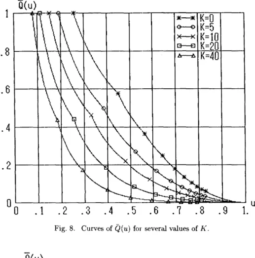
7. Cumulative distribution of u and 1".

Cumulative distribution function of u, the number of observations divided by n, is 1

-Q(u), where Q(11) is given by (2.7). The curve of Q(u) vs. u for the case K = 0 has already been shown (see Fig. 1). Fig. 8 plots the curves of

Q(

u) vs. u for K = 0,5,10,20,40.

Comparison of Fig. 8 here with Fig. 2 of Moriguti (1993b) suggests the smooth transition to the "medium cost" case. This point is made clearer in Fig. 9, in which the abscissa is changed to

u/

j(2K) that corresponds to

11/

y'(2k) in Moriguti (1993b).

Cumulative distribution function F(1") of 1", the absolute rank of the selected object can

be computed with (4.1), (4.6), and cumulative summation of f(1") thus obtained. Fig. 10 plots the F(1") vs. 1" for K = 0,5,10,20,40. (The adjacent points are connected by a line

segment for the sake of convenience.)

Comparison of Fig. 10 here with Fig. 3 of l\loriguti (1993b) suggests the smooth transition to the "medium cost" case. It is seen more clearly in Fig. 11, in which the abscissa is changed to 1"/V(2K) that corresponds to p/V(2k) in \1origuti (1993b).

T(u)

25

20

15

~ ~ ~ I3--£J lr----6

K=O

_I

K=5

K=lO

_~

K=20

J

K=40

10

~

~. ~

~

,

5

"-P--

_~

~

r--

~

~

~ ~ 4?J. -;;:. ~. :~ '~: :

. 1

.2

.3

. 4 .5

. 6 . 7

.8

.9

Fig. 7. Curves of T(u) for several values of K.

8. Final remarks.

1.

u=i

In

The author believes that this paper is in line with the comment by Herbert Robbins on Ferguson (1989).

The gap between the "zero-cost" case and the "medium cost" case has been satisfactorily bridged by this paper. Arguments on "Phase 3" and "Phase 4" in Moriguti (1993b:\ are still applicable, but the author does not think it necessary to repeat the same arguments here.

The results of Moriguti (1992) suggests that "high cost" case will require a little different approach from the other side of the "medium cost" case. We shall leave it to another paper which will follow soon.

Appendix 1. Convergence and The Value of (3.5).

In order to compute the value of (3.5), it is convenient to compute its logarithm first. That is

(ALl) 00 1 8+2

00 _{1 8+1}

loge C(O) =

L

- l o g e -

=

L

- l o g e - '

8=1 8 + 1 8 8=2 8 8 - 1

Incidentally, it is easy to show that (Al.1) is

<

2, using the inequality loge[(8 + 1)/(8 -1)] =

10ge[1 + 2/(8 - 1)]

<

2/(8 - 1) for s ~ 2.

Each term in the right-hand side of (ALl) can be expanded into power series aB (A1.2) 1 8 + 1 2 (1 1 1 ) 00 1

-loge - -

= - -

+ -

+ -

+ . . .

=

2 .

8 8-1 88 383 ₅₈5 _?;(2n-1)82n

Hence the series (ALl) converges like

L

1/82, which is known to be notoriously slow. So we

Secretary Problem with Low Cost

Q(u)

1

~~~~~~~--~--~--.---.--.~~--~ *-*

K=O

~

K=5

~

K=lO

G--EI

K=20

.8~-+-~~~~-+--~--r--+A--h~K=~4*Or-~ .4~--~-~~~+-~~--~~-+---+---+---+-~

00

_{. 1}

_{. 2 . 3 .4}

_{. 5}

_{. 6}

_.7

_{. 8 . 9}

_1.

U Fig. 8. Curves of Q (u) for several values of K.

1

Q(u

_G---€>

_K=5

· 8

~ I3---£l

K=lO

K=20

· 6

• •

K=co

· 4

.2

189

o

0

₁

₂

₃

₄

₅

₆

₇

u*..r(2K)

Fig. 9. Curves of Q(u) vs. u

*

V(2K) for several values of K.

1

F(r)

. 8

_lIr----*

_K=O

~

K=5

~

K=lO

.6

_B----EI

_K=20

lr---A

K=40

.4

.2~~-+----+-·---+----+----;----~--~----·~

r

5

10

15

20

25

30

35

40

Fig. 10. Curves of F(r) for several values of K.

F(r)

1

. 8

V

--v '-' .~

,~

~TO

, 0

0

1(0

0

K=5

1

0

X 0

K=10

K=20

i'

- -

K=co

I

~.

. 6

.4

.2

1

2

3

4

5

6

Fig. 11. Curves of F(r) vs. r/J(2K) for several values of K.

Thus we have (A1.3)

where

(A1.4)

Secretary Problem with Low Cost

00

1

8+1

RN

=

2:

-loge 8 _ 1·

s=N+l 8

Using the well-known formula (A1.5) RN can be expressed as (Al.6) 00

/noo

co

2

x 2n-1 RN =

2:

e-sx ~=

--.

dx s=N+1

a

",=1 2n - 1 (2n - 1)!

ln

oo 00 2 x2n-1 00 =

2: - - .

E

e-sxdx

a

n=l 2n - 1 (2n - 1)! s=N+I

/n

oo 00 2x2n-1 e-(N+I)x - dx - 0

~1(2n-1)!(2n-l)

1-e-x

/n

oo 00 2x2n-1 e- Nx - dx - 0 ;(2n-1)1(2n-1)eX _{-1 .} But (Al.7)

- - = l - - + - : r

x x B12 - - . x + - x B2 4 B3 6 eX - 1 2 2! 41 6! x x 2 x4 x 6

= 1 - - + - - - + - - - · · ·

2 12 720 30240 where Bl, B2,··· are Bernoulli numbers.

Contribution of the second term on the right-hand side of (Al.7) to RN is (A1.8) e- Nx . - d x

/n

00 00 2x2n - 2 -x

a

;(2n-1)1(2n-1) 2 1 00 {CO 2x2n-l =

-2

~l

la

e-Nx (2n _ 1)!(2n _ 1) dx 1 1 N

+

1

=

log -2N eN-I·

Contribution of the rest is

(A1.9)

_la

rx,

00 2x2n-2 [ x 2 x4 x6 ] e-Nx

E

(2n _ 1)!(2n _ 1) 1

+ 12 - 720

+

30240 - ... dx ['Xl [ x2 x4 ] [ x2 x4 ]

=

2

la e-

Nx 1

+

18

+

60ci

+ ... 1 +

12 - 720

+ ...

dx

= 2

_/n

oo

e

-Nx [

1 +

- x 5 2

+

- - - x 53 4

+...

] dx o 36 ]0800 2 5 1 53 1 = N

+

9

N3

+ 225

N5

+ ....

191

Adding (A1.8) and :1..1.9), we get

(A1.10) _{RN =}

_{-"2 .}

1 1 _j\i-loge N _{N _} + 1 _{1 + N} 2 ₊

_9"

5 1 _{N3 + 225} 53 1 _{N5 + ....}

Using the expansion in (A1.3), we obtain a workable formula. For N = 10,20,50, and 100, it yields the same result

(A1.11) loge C(O)

=

1.3531303, so that we get finally

(AL12) C(O) = exp(1.3531303) = 3.8695192.

Appendix 2. Proof of Propositions [5d] Through [5h]

Among the propositions stated in Section 5, Proposition [5d] is indeed the main theorem and all the others are lemmas and corollaries.

First, let us establish the continuity of T'(u). It is obviously continuous in every interval

[us, Us+l)(8

=

1,2,·· .). From (2'.10), we get , 8(8+1), 8

T (u)

=

- - - - 2 - - K

+

-2uT (u) (us:S u :S Us+l).

2u u (A2.1) Considering (2.14), we obtain (A2.2) T '( _US

₊

0)==-8(8+1)_K' ₂

₊

~_8(8-1)_K'

_{2 - 2 '} 2us Us 2us and (A2.3) T'( Us+l _ 0) - -8(8 + 1) _ - 2 K

+

8(8 + 1) _ 8(8 + 1) _ 2 - 2 K' .

2us+l us+l 2us+1

Thus we have

(A2.4) T'(u s

+

0) = T'(u s - 0) (8 = 1,2,·· .),

which means that T'(u) is continuous also at the boundary points. So it is continuous everywhere in the interval (0, 1).

Since T'(uIl = -K

<

0 and T'(u s)

>

0 for sufficiently large value of s (e.g. for 8 =

1 + J(2K)), there must be at least one point u in the interval (Ul' 1) where T'(u) =

o.

This is a part of the "Theorem" [5d].

If it lies in the interval [us, Us+l) where 8 ~ 2, then (2.10) gives us (A2.5) T( -) _ _{u -}

!!.

[8(8 ₂₂

+

1)

_+K,

]

8 u and substituting it into (2.12), we get

(A2.6) - - - + K = - - - + A 1it[8(8+1)"] 8 K 1

Secretary Problem with Low Cost 193

that is

(A2.7) As = ( 1 )_ +1 [2Ku --2 8(8 - 1)]. 28 8 - 1 US

On the other hand, (2.12) and (2.14) gives us

8 8 K 1 1 [ ' 2

A, = - us+! + 2us+1 + 8 _ 1 ~'-1 = 2(8 _ l)us+1 2Kus - 8(8 -1)],

S S .Il S

(A2.8) and

(A2.9) _As

₌

_--.s:tT+

8+1 2 8 s+1

+

-'-1' K s-1 1

=

2( 1 . 1) s+1[2Kus+1 - (8+2)(s--I)]. , 2 .

11s+1 11s+1 s - U_s+l 8 - 11s+1

The ratio of (A2.8) to (A2.7) gives us (5.9), and the ratio of (A2.9) to (A2.7) gives us (5.10). Proposition [Se] is thus proved. Proposition [Efl is similarly proved, using (2.13) in place of (2.12).

Now we have come to the point to prove the remaining part of "Theorem" [5d], that

T(u) has a unique minimum at

u.

If u lies in the interval [us, us+d and 8 2: 2, then substituting (A2.7) into (2.19) we get (A2.10) " S u

s

-2 -2

T (u)

= - -

-_--[2Ku - s(s - 1)].

u3 _2us+1

On the other hand, since s = int[uT(u)], we have (A2.11) s ~ uT(u)

<

8 -+-1,

and (A2.5) together with this gives us

(A2.12) S(8 - 1) ~ 2Ku2

<

8(S

+

1). At U, (A2.10) becomes (A2.13) -s-2 T "(-) 11 = -S - - -U [K'-2 2 11 - s( . 8 - 1 )] u3 2us+! .

=

2~3[28

- {2Ku2 - s(s - I)}]

=

2~3[S(8

+ 1) - 2Ku2],

and we get T"(u)

>

0 because of (A2.12). Hence if T'(u)

=

0, then T(u) has a minimum there.

If

u

happens to coincide with Us, then we have to carry out more manipulation. Since Us is at the lower end of the interval [us, Us+l), the above argument tells us only that if T' (us) = 0 then

(A2.14) T"(us

+

0)

>

O.

Considering the limit, as u -+ Us - 0, of (A2.13) after replacing 8 by s - 1, we get when

u

=

Us

(A2.15) T"(us - 0) = 213[(S -1)8 - 2Ku;] = O.

This is short of what we would hope for. But, replacing s by s - 1 in (2.19) and using (A2.5), we get

(A2.16) _As-I

₌

_{(s _ 2)u:+l} 1

_>

_o.

Then, from (5.1) and (A2.9), we have

(A2.17) T ",( u)

=_.

:3(s-1) 4 -A_s-I(S-1)(s-2) s-3)u ( 8 - 4

u

<

0 (Us-I::; U

<

Us,S ~ 3).

Therefore, at least for sufficiently small h

>

0, we obtain

T'(us - h)

=

T'(us ) - hT"(us )

+

~~

T"'(us - Oh)

<

0,

where 0 is between 0 and 1. This result, together with (A2.14), will assure us that, even if

ii

=

Us, T(u) takes a minimum at

u.

When

u

lies in the interval [ut, U2), then we must use (2.20), (2.21), (2.22) in place of

(2.17), (2.18), (2.19). But (A2.1) still holds here. Therefore, if (A2.18)

then 1 = int[uT(u)] implies (A2.19) and consequently (A2.20) Now (2.22) gives us (A2.21) 1 1 T'(u) = - -2 - K

+

-2 uT(u) = 0, u u 1 ::; uT(u)

=

1

+

Ku2

<

2, 1-Ku2

>

o.

T" (u)

=

:3

(1 - Ku2)

>

O. U

Since T'(UI - 0)

=

-K

<

0, there is no problem even if

u

=

UI.

Only remaining point is what will happen if

u

=

U2. In that case, (A2.14) still holds when s

=

2. In stead of (A2.13) with s replaced by s - 1, we have to use here (2.22) which gives

(A2.22)

On the other hand, we get from (2.21) that, if T'(U2)

=

0 then (A2.23) whence (A2.24) Al

=

-212 - K(loge U2

+

1), u2 '( 1 1 " u T u) = - . -

+ -

+

Klog -

<

0 if u

<

U2. :2u2 _{2u~ e U2}

Secretary Problem with Low Cost 195

This will suffice to complete the argument above when

u

=

U2.

Now we are ready to complete the proof of the remaining part of "Theorem" [5d], that is the uniqueness of the point u where T'(u) =: O. Through a rather lengthy arguments, we

have established the "Lemma":

(A2.25) If T'(u)

=

0 then T(u) has a minimum at u.

As T'(u) exists and is continuous in the whole interval (0,1), at a point where T(u) has a minimum or a maximum, T'(u) must be zero. But (A2.25) prohibits the existence of a maximum. If there were more than one minima, then there would be a maximum between two adjacent minima, which is impossible. Therefore there can be only one minimum. This completes the proof of "Theorem" [5d].

Let the unique minimum of T(u) be in the interval [us., us.+I), then (A2.12) tells us that 2Ku2 - s·(s· - 1) ~ 0, and consequently 2Ku; - s(s - 1) ~ 0 for s

=

s· thanks to

(5.9). Now, [5b] will produce

(A2.26) 2Ku; ~ s(s-1) for s

=

s·,s· -1,···,1. Next, (A2.12) tells us that 2Ku2

- s*(s·

+

1)

<

0, and consequently 2Ku;

<

(s

+

1)(s - 2)

for s

=

s·

+

1 thanks to (5.9). Then [5c] will produce

(A2.27) 2Ku;

S

(s

+

1)(s - 2)

<

s(s - 1) for s

=

s*

+

1, s· + 2,···. This completes the proof of Proposition [5g].

Proposition [5h] comes from the fact that s* is the greatest integer satisfying s(s - 1) S

2Ku2.

REFERENCE~S

[1] Chow, Y.S., Moriguti, S., Robbins, H. and Samuels, S.M. (1964) "Optimal selection based on relative rank (the 'secretary problem')" Israel Journal of Mathematics Vol. 2, 81-90.

[2] Ferguson, T.S. (1989) "Who solved the secretary problem" Statistical Science Vol. 4, 282-296.

[3] Moriguti, S. (1992) "A selection problem with cost - 'secretary problem' when unlimited recall is allowed" J. of Operations ReseaT·ch Society of Japan Val. 35, 373-382.

[4] Moriguti, S. (1993a) "Basic theory of selection by relative rank with cost" J. of Opera-tions Research Society of Japan Vol. 36, '*6-61.

[5] Moriguti, S. (1993b) "Asymptotic theory of selection by relative rank with medium cost" ,

J. of Operations Research Society of Japan Vol. 36,102-117.

Sigeiti Moriguti Syoan 2-16-10 Suginami-ku Tokyo 167, JAPAN