Optimal Tool Module Design Problem for NC Machine Tools

Society of I apan

Vol. 27, No. 3, September 1984

Abstract

OPTIMAL TOOL MODULE DESIGN PROBLEM

FOR Ne MACHINE TOOLS

Ryuichi Hirabayashi

Tokyo Science University

Hisatoshi Suzuki

Tokyo Institute of Technology

Noboru Tsuchiya

Hitachi Production Engineering Research Laboratory

(Received September 21,1983: Final March 15, 1984)

In order to enhance factory automation and unmanned production, numerical controlled (NC) machine tools are widely used in many mechanical processing factories. Whenever one machining part is changed to another, the operation of an NC machine tool has to be stopped in order to change some of the cutting tools on the turret tool holder. In this paper, a new concept of 'tool module' is used and the problem of reducing the number of tool changing operations for Ne machine too\:; is discussed. The problem is formulated as a 0-1 integer programming (0-1 ILP) problem on a bipartite graph and a branch and bound algorithm is proposed to select an optimal tool module. Since the LP relaxation problem obtained by dropping the integrality condition for the 0-1 ILP problem has a special network structure like the well-known transportation problem, this LP is solved by certain network flow algorithm with utilizing its special structure Some numerical experiments are reported, and indicate that the algorithm is reasonably efficient. Furthermore, possible extensions of this method are discussed.

1.

Introduction

Recently, a lot of numerical controlled machine tools (briefly, Ne machine tools), such as machining centers and turret punch presses, have been introduced in many mechanical processing factories. Nowadays, Ne machine tools are indispensable to high quality and high efficient production. Since a worker can handle several Ne machine tools at the same time, it is possible to reduce man-hours and lead-times greatly. Thus, Ne machine tools are useful to achieve the factory automation as well as the unmanned production, which in turn increases the produc-tivity. These bring an innovation in the aspect of factory management.

206 R. Hirabayashi, H. Suzuki and N Tsuchiya

of cutting-tools play an important part in the productivity improvement. Hence, our main attention is paid to the tool changing operations and reduce the number as much as possible. In this paper, this problem will be treated as a mathematical programming problem.

In the succeeding sections of this paper, mainly the machining center is considered. However, the similar procedure is adaptable for many other types of NC machine tools. At a machining center simul-taneously several cutting-tools can be installed such as face cutters, drills, endmills, taps and so on, with the range from 12 to 80 for each NC machine tool (the maximum size of tool magazine is a constant for each NC machine tool). Usually, for processing one part, only 40 - 60% of installable tools are used. Moreover, some of these tools are common for processing different kinds of parts. Hence, we consider a produc-tion method based on the group technology concept. In this method, all parts are partitioned into several groups, and each group is called a "parts-family". The parts contained in each family may require a lot of processing tools in common and can be processed by the same set of tools within the maximum size of tool magazine. We call this set of tools as a "tool module", and when a parts-family changes, whole set of installed tools i.e., a tool module is changed. Therefore, the number of set-up operations is the same as the number of parts-families (i.e., the least number of tool modules needed for processing all parts). Thus, if we construct some suitable tool modules, the total set-up operations will reduce considerably.

We denote by

M

{1,2,···,m} the set of tools, by N

=

{1,2,···,n} the set of parts to be processed and by E E M x N the relation between

tools and parts, i.e.,

(i,j)

E

E

means that the tool

i

is used to pro-cess the part j. Let a positive integer k be the maximum size of tool magazine. Then, the problem mentioned above can be restated as follows; cover

N

by the least number of parts families each of which can be processed by one tool module with at most

k

tools. We call this problem as the

optimaZ parts grouping probZem

(OPGP).

The OPGP was first studied in IS]. If

I(j)

be a set of tools necessary for processing the part j and

II(j)1

be the cardinal number of

I(j),

the Hamming distance

d ..

between

i

E Nand

j

E

N

is defined by

d ..

~J ~J

= II(i)

EB

I(j)

I

= II(i)

I

+

II(j)

I -

2II(i) n I(j)

I.

In IS], using this Hamming distance as a metric, several heuristic methods for parts group-ing methods were proposed, namely, if d .. is large, then

i

and j should

~J

belong to different families. Conversely, if d .. is small, then

i

and j

should belong to the same family. In this situation, each parts-family should require at most

k

tools for processing.

In this paper, given a profit 1T. (nonnegative) for each part j (j J

1,2,···,n), we consider a problem to construct an optimal tool module that maximizes the profit. We call this problem the

optimal tool module

design problem

(OTMP). Initially, this is considered as a problem on a bipartite graph and subsequently converted to a 0-1 ILP problem. Let 11. = 1 for every j EN, then the OTMP h to find a tool module which

J

maximizes the number of parts to be processed by it. Let 1T. be the pro-J

cessing time of part j, then the problem is to find a tool module so as to maximize its continuous utilization during processing. The latter problem is very important for unmanned night shift production.

So far we have discussed the OTMP i.nstead of analyzing the OPGP directly. By the following two reasons, it can be shown that the former consitutes a subproblem of the latter. If we can obtain an optimal tool module for given

M

and

N,

then by deleti.ng from

N

the parts which can be processed by the tool module, the next OTMP for M and the remaining N is determined. Repeating this procedure until

N

becomes empty, we can get a sub-optimal solution for the OPGP. The second reason is that the OPGP can be formulated as a set covering problem and that the OTMP is useful to generate coefficient column vectors of the set covering problem. More details are stated in the last section of this paper. Thus, it is valuable to study the OTMP to solve the OPGP as the first step.

2.

Description of the Problem

Given a bipartite graph (J.j,N,E), where M U,2,···,m}, N

=

{l,2,

···,n}

and E C M x N, we define ICj)

=

fi EM (i,j) E E} for each j EN. Let k be a given positive integer and 11. Cj E N) be nonnegative

J

constants. Then we consider the followi.ng problem (see Figure 1):

maximize

L

11 • I(j)cS J

subject to

S C M,

Isl ::;

k·

Reading

M

as the set of tools, as

N

the set of parts,

E

as the binary relation E = {(i ,j) E M x N I the processing part j needs the tool i}, k as the maximum size of tool magazine for a machining-center

208 R. Hirabayashi, H. Suzuki and N. Tsuchiya

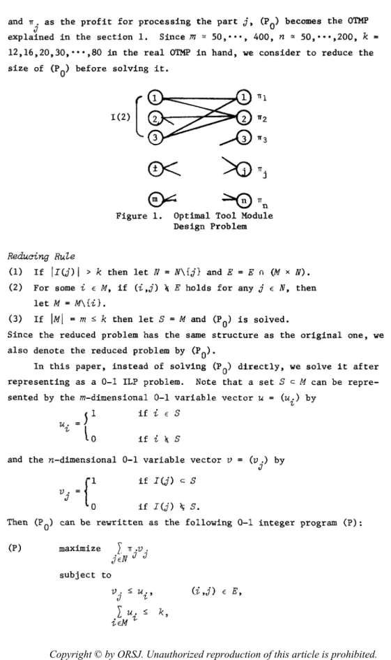
and ~j as the profit for processing the part j. (PO) becomes the OTMP explained in the section 1. Since

m

~ 50,···, 400,

n

~ 50,···,200, k 12,16,20.30,···,80 in the real OTMP in hand, we consider to reduce the size of (PO) before solving it.

1(2) [

~ ~~n

Figure 1. Optimal Tool Module

Design Problem

Redueing Rule

(1) If /I(j)

I

> k then let N

=

N\{j} and E

=

E n (M x N).

(2) For some i E M, if (i.j) \ E holds for any j E N, then let M = M\{iL

(3) If

/M/

= m

~

k

then let

S

=

M

and (PO) is solved.

Since the reduced problem has the same structure as the original one, we also denote the reduced problem by (PO)'

In this paper, instead of solving (PO) directly, we solve it after representing as a 0-1 ILP problem. Note that a set S c M can be repre-sented by the m-dimensional 0-1 variable vector u

=

(U

i ) by

U. =

5

1

1-

lo

i f

i

E S

i f i 11; S

and the n-dimensional 0-1 variable vector v

i f I(j) c S

i f I(j) l!;: S.

(v.) by

J

Then (PO) can be rewritten as the following 0-1 integer program (p):

(p) maximize

2.

~.v. jEN J J subject to Vj ~ u

_{i '}

L

u. ~ k, iEM 1-(i,j) E E,

U. E {O,ll, '/-V. E {O,ll, J

i

EN, j E

N.

In the problem (P), when we determine the value for the vector U, the vector V is determined automatically by V. = min

u.

for all j E

N.

J (i,j)EE

'/-Therefore we can consider that the essential variable vector is u. Thus it is clear that the constraints V. E {O,l}, j E

N

can be omitted.

J

3. Branch and Bound Method

In this section we will describe a branch and bound algorithm for solving the problem (p). We will denote by SP(t) the subprob1em on the t-th node. Let Also, Here, let IO {i E M I1 {i E M

r

{ i EM u. '/- is fixed at U. is fixed at

'/- °

1 u.~ I u I }.

'/-°

in the t-th node}, 1 in the R,-th node},

JO U J(i) u {j E NI j E J

°

for the parent node} , idO

J1 _{{j E N I(j)} c I1} u {j _{E N}

I

j E J 1 for the parent node} ,

~

{j E N

I

j

~

JO u Jl}.

J(i)

=

{j E N

I

(i,j) E El. Since V.

J

optimal solution of SP(t) satisfying

min

u

_i ' there exists an i d ( j )

Vj {

i f j E J 1 ..

t

Hence, letting

E

E n {(i,j)

liE

r,

j

E

~},

the subprob1em SP(R,) is: SP(R,) maximize

L

n.V.

+

L

n. . y J J • JO J subject to JE~ JE t (i ,j) E E , k -

l.rll,

210 R. Hirabayashi, H. Suzuki and N. Tsuchiya

U. E {O,ll,

"I-

i

E

r.

Also, we will denote by SP(~) the LP relaxation problem of SP(~) and by z(~) the objective function value of SP(~). The algorithm for solving SP(~) is described in the section 5.

We will consider (PO) to get an i.nitial feasible solution. Without loss of generality, we can assume n

l

~ n

2

~

•••

~ nn' Then, let 8

=

I(l)

first, and, for ~

=

2,3,···,n

in order, let 8

=

8 u I(~) if 18

u I(~)I ~

k.

The resulting 8 is a greedy solution for (PO)' There are some other heuristics to find initial feasible solutions of (p) or (PO)' Clearly,

u

_l

_{=u 2="'=Uk=1, uk+l=Uk+2="'=Un=0}

is a trivial initial feasi-ble solution. Another heuristic to find a feasible solution is as follows. Select some

j

E N and let 8

= I(j).

The set I(~), ~ E N, with the nearest Hamming distance to 8 has priority to join with 8 (i.e., 8 is replaced with 8 u I(~» and repeat this process as long as 18 u I(~)I ~

k.

Branah and Bound Algorithm.

(step 1) Find an initial feasible solution of (p) and obtain

zI

the corresponding value of the objective function. Let ~

=

1 and all ui's,

v.'s

be undetermined, i.e.,

r

=

M

(~becomes

N) and SP(l) is equal to

J

(p). Let the active node set

N

=~. Reduce SP(l) by the following reducing rule.

Reducing Rule

(1) For every

j

E

~

such that

II(j)

n r l >

k -

IIll, let

v.

JO u {j},

.1

=

.1\

{j} and

E~

=

E~

\

(I(j)

x

{j}).

J (2) (3) (4) (5) (6) For every j E

.1

and

.1

= .1\{j}.

such that

I(j)

n

r

~,

let

v.

J

For every i E r such that J(i) n

~

and

r

=

iF\{i}.

~, let u.

1.-For every i E r such that

.1

c J(i), let u. 1.-r

=

r\{i} and

E~ = E~

\ ({i} x J(i».

For every

j

E

.1

such that

II(j) n

r l

=

k -

IIll, let 8

=

I(j) n

r

and set

z(~)

=

I

n

+

In.

In the case

z(~)

>

Ji'

P

lP

I I(p)nTc8

P6

J

°

zI,

let

z

=

z(~).

Let V.

=

0, J

= J

u

{j},

.1

=

.1\{j}

and

E~

=

E~

\

(I(j)

x

{i}).

J If Irl

~

k - IIll

r=

lA then let u• .F

i

p,

v.

=

1 for any J E J , J

=

1 for any

i

E

r,

Il

=

Il

u

r,

Jl

= Jl

u

~, ~

=

~

and set

z(~)

=

z(~)

=

I

In ..

In this case SP(l) is solved.

Reconstruct the subproblem SP(l)

~

and Et. Solve the relaxation

. 0 1 -F 0 1

by us~ng the new I • I , 1~ ,

J , J ,

I

z

then go to step 6. If z(l)

problem SP(l) and get

z(l).

If

z(l)

$

I

>

z

and all

u.

I s and V • I S are integer

1.- J I

values, then let z

z(l)

and go to step 6. Else record all

ui's, Vj's

and Z(l) at the node 1 and let

N

=

{I}.

(step 2) If

N

=

0

then go to step 6 else select the node p which is lastly generated. If

z(P)

$

zI

then

N

=

N\

{p} and return to the top

of step 2.

(step 3) Select a

u

_i

which is fractional in the node p. Then, we will fix the variable u. to

a.

which is either 0 or 1. If both 0 and 1 are

1.-

1.-already used to fix u. then let

N

=

N\

{p} and go to step 2. If u. can

1.-

1.-be selected then fix u

_i

=

ai'

let ~

=

~

+

1, generate the subprob1em SP(t), record it to the node t and let N

=

N u {R,}.

(step 4) Reduce the subprob1em SP(t) by the reducing rule described in step 1 and reconstruct

SP(~)

by using the new IO, •••

,~.

Solve its relaxation Sp(t) and obtain the objective value

z(t).

Record all values of

u.'

s and V • 's at the node t.

'l- J

(step 5) In the case of

z(t)

$

zI,

let

N

=

N \

{t} and go to step 2.

- I

In the case where z (t) > z and there exist a fractional u" go to step

_ I 1.- I

2. In the case when

z(t)

>

z

and every

u.

is integer, let

z

=

z(t),

1.- I

delete all nodes t' E N from N such that z(R,') $

z

and go to step 2.

(step 6) The present value

zI

is the optimal value for the original problem (p) and the solution which gives the objective value

zI

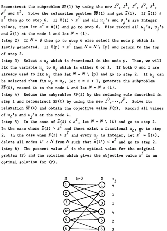
is an optimal solution for (p).

M k=3 N 5 1 4 2 3

Figure 2. An example of the Optimal Tool Module Design Problem

212 R Hirabayashi, H. Suzuki and N. Tsuchiya

Consider the OTMP given by Figure 2. The result of the branch and bound method is given by Figure 3. In this example, the initial

solu-I

tion is

S

=

1(2)

= ll,3,S} which is a greedy solution and

z

= S. At node 1, by the reducing rule S described in the branch and bound algo-rithm, JO becomes {2,4}. Then by the reducing rule 3, 1° becomes {3} and the reduced subproblem SP(l) is illustrated as Figure 4. Solving SP(l), we get z(l) = 27/4, U = (3/4,3/4,0,0,3/4,3/4) and V

(3/4,0,0,

0,3/4,3/4).

At node 2, we fix

u

_l at 1, then 11 is {I} and k_IIll becomes 2. Hence, by reducing rule S, we have the new integer solution

u

= (1,1,0, 0,1,0), V = (1,0,0,0,1,0) and the objective function value

z

= 6. Since

I I

°

z

>

z ,

we replace

z

by

z

(= 6). J is now {2,4,S}. Next, applying the reducing rule S again to

6

E

~

= {1,3,6}, we have 11 =

{I},

1° =

1

°

{3}, J

0

and J = {2,4,S,6}. Now apply the reducing rule 3 and we have 11 {l}, 1° = {3,s,6}, Jl =

0

and JO = {2,4,S,6L Since 11'1 =

1{2,4}1 2 =

k -

1111, by reducing rule 6, 11 becomes {1,2,4} and

z(2)

=

z (2)

=

s.

I

10=3,

° { }

1 d I d Z =S, J

=

2,4 , I =v, J =v,

z=27/4, u=(3/4,3/4,0,0,3/4,3/4),

V=(3/4,0,0,0,3/4,3/4)

I I z =6, z=S, z =6, z=S, u=(O,l,O,O,l,l), u=(l,l,O,l,O,O), v=(O,O,O,O,l,l) v=(l,O,l,O,O,O) optimal solution; z=6, u=(l,l,O,O,l,O), v=(l,O,O,O,l,O) Figure 3. Result of 'the branch and bound

algorithm for the problem in Fig.2

°

°

At node 3, since we fix

u

l at 0, I = {1,3} and J = {1,2,3,4}.

°

1

Then by the reducing rule 3 and 6, we have I = {1,3,4}, I = f2,S,6},

I'

=

0,

J

O

= {1,2,3,4}, Jl {S.6},

~

=

0

and

z(3)

=

z(3)

= S. Since both node.2 and 3 are fathomed, the active nodes set becomes empty and the algorithm terminates. The optimal solution obtained isu = (1,1,0,0,1,0), v = (1,0,0,0,1,0) and the objective functional value is 6.

4.

Relaxation of the Problem (P)

Now, let us consider a subproblem eof (p) where some

Ui's

are fixed at either 0 or 1. Since such problem has the same structure as the original one as shown in the section 3, we will study the structure of (P) instead of those of its subproblems.

Consider an LP-relaxation problem

(P)

of (P): Maximize

I

1I.V.

jEN

J J subject to

V.

::; u. J

t-I

u. ::;

iEM

t-O ::; u. t-O ::;

_v.

J

(i,j)

E E,

k,

::; _{1, i E M,} ::; _{1, j E}

_N.

As in the problem (P), we can omit the constraints 0::;

Vj ::;

1,

j EN

from

(P).

On the other hand, let x

=

(x .. )

(i,j)

E

E

be the Lagrangean

t-J

variable vector for the constraints

Vj ::;

u

_i

' (i,j)

E

E

and consider the Lagrangean relaxation problem:

maximize

I

1I.V. -

LX . .

(v. - u.)

jEN

J J

(i,j)EE

t-J J t-subject to

I

u. ::; k,

iEM

t-u. E {O,U, t-V. E {O,U, J i E M, j E

N.

Let us denote by 2(') the maximal Then 2(P) ::; 2(L ) for any x ~ 0 holds

x

objective value of a problem ('). in general, and min

z(L )

gives

>0 x

the best upper bound of z(p) [1). We will show that t~e next theorem holds;

Theorem 1.

min 2 (L )

=

2 (p) .

x~O x

Proof:

2(L )

=

x

maxI

_jEN

L

1I.V. -

_{J J}

_(i,j)EE

LX . .

_t-J (v. -_J u.) _t-

I

_iEM

I

u. ::; _t- k,

U. E {O, l} (i E M),

v.

E {O, l} j EN)}

t- J

max{

L

(11. -

LX .

.)v .

+

I ( I

x .. )u.

jEN

J

iE](j)

t-J J

iEM jEJ(i)

t-J

t-214 R. Hirabayashi. H Suzuki and N. Tsuchiya

L

u. s k, u. E { 0 , I} (i E M), V. E {O, I} (j E N)} i E M " l - " l - J maxi

L

(1T. -

L

x .. )v.

+

L ( L

x .. )u.

I

j d J iJ~)~ J i~j~U)~

"l-L

u. s

k, 0

s u.

~ 1 (i E M), 0

s

V.

s

1 (j E N)} i E M " l - " l - J max{

L

1T.V. -

LX . .

(v. - u.)

I

L

u. s k, jEN J J (i,j)EE"l-J J "l- i~

"l-o

S

u. s

1 (i E M), 0

s

V.

s

1 ~ E N)} "l- J z (Lx)'

where (L ) is the Lagrange relaxation problem for

x (p) • Moreover, since

(P)

is an LP problem, min

z(L )

x~O x min z(L )

=

min

z(L )

x~O x x~O x z (P). Therefore, z (P).

By this theorem, it is verified that

z(P)

gives the best upper bound for

z(p) in the sense of Lagrange relaxation.

0

Next we will

(P).

For solving

E),

A,

~i (i E

M)

problem

(P):

discuss a method solving for the LP-relaxation problem

(P),

let us introduce the dual variable x .. «i,j) E "l-J

and construct the dual problem

(D)

of the primal

(D) minimize kA

+

L~. subject to iEM

"l-L

x .. -iEI(j) 1-J 1T j ' j E N,

L

x ..

s

_A

₊

_~i' i E M, jEJ(i) "l-J x .. ~ 0, (i ,j) E E, "l-J A ~ _0, ll· ~ 0 i E M.

"l-For the optimal solution of

(D),

the next theorem holds;

Theorem 2.

Let

(x*,A*,ll*)

be an optimal solution of

(D).

Suppose

L

x.*

jEJ(l) 1j holds, then A*

L

Xkj*' jEJ(k)

LX,,* -

A* jEJ(i) 'Z-J

°

i f

i ::;

k for all

i

E M, i f

i

> k

holds and the optimal value of objective function is given by

k k

z (D)

L LX"*

=

1.

(A~'

+

].1.*).

i=l jEJ(i) 'Z-J i';l "/..

Proof:

Let~.

L

x ..

*

fo'(' eVE'ry

i

E M, then (A*,].I*) should be "/.. jEJ(i) "/..J ~

an optimal solution of the next problem (D):

~

+

L].I·

(D) minimize kA subject to iEM "/.. A

₊

_].Ii ~ _~i ' i EM, A ~ 0, ].I. ~ _{0, i} E M. "/..

Let A* ~k and, for every i E M,

= {:i

- ~k i f i ::; _k ].1.*

"/..

i f i > k

then, since ~1 ~ ~2 ~ ••• ~ ~ ~ 0 holds from the assumption of the

n ~ ~

theorem, (A*,].I*) is a feasible solution of (D). The dual problem (p) of the problem (D) is:

(P) maximize subject to

By the condition _~1 optimal solution and

=

{1

u.*

"/.. 0

L

~.u. iEM "/.. "/..

L

u. ::;

k, iEM "/..

°

::; u.

::; _1, "/.. ~ _~2 ~

...

~ the optimal i f i ::; _k i f i > k k i E M.

~ ~ 0,. it is easily seen that the

n

value of (p) are

for all i E M,

z (P)

L

~.u.*

L

~

..

216 R. Hirabayashi, H. Suzuki and N. Tsuchiya

k

Since

kA*

+

L

~.* =

L

a. =

z(P),

by the duality theorem (A*,~*) is the

iEM 1.- i=l

1.-optimal solution of (D).

0

Corollary 1.

Let

A

=

Cl/m) L~' and ~i = 0 for every

i

EM. If

jENA

J

A

there exists a feasible flow vector:x: = (x .. )

A A 1.-J

(M ,N ,E) such that

LX..

$ A,

i

E M and

x..

~

jEJ(i)1.-J 1.-J

on the bipartite graph

A

0, (i,j) E E, then (X, A,~) is an optimal solution of the dual problem

(D).

Proof:

It can be easily shown that

(X,A,V)

is a feasible solution

of (D) and the objective value is

k~

+

L~'

=

(k/m)

L

~

..

On the

iEM 1.- jEN J

other hand, let (X*.A*,~*) be an optimal solution of

(D)

and, for simplicity, satisfy the assumption of Theorem 2. Then, by the Theorem

2,

k

z

(D)

L L

_{x ..}

*

i=l jEJ(i) 1.-J

~ (k/m)

L L

x ••

*

iEM jEJ (i) 1.-J

(k/m)

L L

x ..

*

jEN iEI(j) 1.-J

(k/m) L1T .•

jEN J

Hence, (X,A,~) is a better feasible solution than (X*,A*,~*). Therefore

A A A

(X,A,~) is an optimal solution of

(D).

0

5. Algorithm for solving

(5)

In this section we will describe a primal-dual algorithm (see, for example [4]) for solving

(D).

Adding two nodes U

_o

and VO' (p) can be reformulated as the following problem

(P'):

(p') maximize L1T.(V.-V O) jEN J J subject to

L

Cu

_{o -}

u.) ~ m - k, iEM 1.-U. - V. ~ 0, 1.- J U

_{o -}

u

i

~ 0, Vj-VO~O, U

_o

= 1, Vo = O. (i,j) E E,

i

E

M,

j E

N,

(p') can be regarded as a projeat saheduUng prob~em with an additional linear constraint and can be solved by a general solving method deve-loped in 12,3]. There, k is treated as 11 parameter and (P') is solved

parametrically from

k

=

m-I

to

k

=

k.

The algorithms developed in 12,3] are for general network programming, hOWE!ver, (P) has a more simple structure as a bipartite graph. Therefore, we develop a simpler primal-dual algorithm for

(P)

and

(D)

in which ~: is regarded as a fixed scalar.

In order to solve

(D)

by using the primal-dual algorithm, it is enough to fjnd a solution (u,v ,.:.c,A ,11) satisfying the primal feasibility;

(5.1) (5.2) (5.3) the dual (5.4) (5.5) (5.6) (5.7) (5.8)

v

j -

u

_i !> 0,

L

U. !> k,

iEM

1.-°

!>

u

_i !> 1, feasibility;

L

x ..

iEi(j)1.-J

L

x .. !>

jEJ(i)1.-J

x .. 2: 1.-J A 2: 0. 11· 2: _0, 1.-(i ,j) E E,

i

E M" j E N" A

+

11i' i EM" 0, (i ,j) E E,

i

E M" and the complementarity condition;

(5.9) (5,10) (5.11) (5.12 ) (v. - u.)x .. J 1.- 1.-J

( L

u. -

k)A

iEM

1.-°

(i,j)

E E, 0,

°

i EM" - (A+I1.»U. 0, i: EM. 1.-

1.-We first construct an initial solution (U,V,x,A ,11) which satisfies the conditions (5.1)-(5.12) except (5.9) and modify the solution until the solution satisfies all the conditions (5.1)-(5.12).

In the rest of this section we will discuss a primal-dual algorithm to solve

(D).

Let us define the notation k-max which is used in the algorithm. Given the constants a

l,a2,···,a

_p

'

we will denote by k-max{ai

i

= 1,2, ••• ,p} the k-th largest number in the set fa

l, a2, " ' , ap}' I f a

l 2: 02 2: ••• 2: a_p' then k-maxfa

_i

I

i

=

1,2, •••

,p}

=

a

_k

.

Before des-cribing the algorithm completely, we will explain the outline briefly. In the step 2 of algorithm D, using the present flow

<.x •• ),

the dual

1,J

variables A, 11 are determined naturally by Theorem 2. u

218 R. Hirabayashi. H. Suzuki and N. Tsuchiya

is determined by (5.11) and (5.12), while the remaining u

i

(i

E Ip) is

averaged so that it may satisfy (5.2) and (5.10). Thus it can be seen that except (5.9) all other equations (5.1)-(5.12) hold. On the other hand, by Corollary 1,

L

::c • • will be optimal i f i t is equal to

Z.

jEJ(i) 1-J

Hence, in the step 3 - step 8, we will try to make

L

::c •• jEJ(i) 1-J

to be

z.

Here, cr. and T. are labels for

i

E

M and

j EN respectively. cr.

=

-1

1- J

1-(T

j = -1) means that i E M (j E N) is unlabeled, while cri ~ 0 (Tj ~ 0)

means that i E M (j E N) is the labeleQ state. In the step 10, we

examine each node i E I whether it is necessary or not to change

L

x .. jEJ(i) 1-J by using the present values of labels cr.

(i

E

I).

1-Algor>i

trun

D.

(step 1) For each j E N, select iO E I(j)

for all other::c .. , (i,j) E E. Let I = M.

1-J (step 2) Find A

=

k-max{

I

x .. jEJ(i) 1-J

I

i EM}, I = 0 {i E I _jEJ(i)

L

::c •• < _1-J A} , I = {i E I

L

::c •• > A}, 1 _{jEJ(i) 1-J} I = {i E I

L

::c •• A} , F _{jEJ(i) 1-J} II .

=

max (0,

L ::C .. -

A), 1- _{jEJ(i) 1-J} and let::c . . 1-oJ i E M, 1 i f i E I l "IT. and::c .. J 1-J

u.

(k _IIll)fIIFI i f i E IF for every i E I,

1-0 i f i E IO

v.

= min {u. l i E I(j)}, j E

N.

J

1-o

If

(v. - u.)x ..

=

0 are satisfied for all (i,j) E

E,

then go to step 11. J 1- 1-J

(step 3) Let

i

=

I

L

::c •• / III i d jEJ(i) 1-J and S -:

L::C" -;,

i

E I. " jEJ(i) 1-J (step 4) Let

"i

-f'

-1 i f S. > 0 1-otherwise for each

i

E

I.

If cr. -1 for all

i

E I then go to step 9. Otherwise, let

1-T. = .1 s. = 1.--1 S. 1.-j E

N,

for

i

E J and S. > O. t

(step 5) For every

i

E I which has become i f there exists j E J(i) such that T.

=

-·1

.1

cri ~ 0 in the previous step, and x .. > 0 then for all j E

1.-.1

J(i) satisfying the condition, let tj = min(x .. ,s.) and T. =

i

else go 1.-.1 1.- .1

to step 9.

(step 6) For every j E

N

which has become T. ~ 0 in the previous step, .1

if there exists i E I(j) n I such that cri = -1 then for all i E I(j) n

I satisfying the condition, let S..

t.

a.nd cr ... j else go to step 9.

v .1

1.-If a node i E

I

which satisfies

Si

> 0 is found above then let io = i,

8

= min (s. ,-S.), .10 .70 else go to step 5. (step 7) Let j 0 = cr. , .10

x . .

=X • • +s, 1.-clo 1.-clo

If cr. > 0 then repeat step 7 else go to step 8. 1.-0

(step 8)

(step 9)

Let S.

=

S. - s and go to step 4. 1.-0 '1-0 Find >.. = k -max {

Lx..

l i E M}, jEJ

(0

1.-.1 IO {i E I

I

L

x .. <

>"},

jEJ(O 1.-.1 I1 {i E I

I

L

x .. >

>"},

jEJ(i) 1.-.1 Ip {i E I

I

L

x ..

>"},

jEJ

(0

1.-.1 11 • = max (0,

L

X •• - >..), i EM, 1.- _{jEJ(i) 1.-.1}

=f~

i f i E ₁₁ u. - 111

u

{i E M

I

i

\

I and u. = 1.- 1-i f i E IF 0 H i E I O' 1}

I) /

IIp

I

220 R. Hirabayashi, H. Suzuki and N Tsuchiya

V. = min {u. l i E J(j)},

J 1.- j E

N.

For every (i ,j) E E, i f (V. - u .)z ..

J 1.- 1.-J

o

is satisfied, then go to step

11. (step 10)

let J

=

{i E J I cri ~

a}.

let J = {i E J I cri

=

-I}.

3) In the case where A =

it

and I{i E MU I u. UI

1.-1) In the case of A > x,

2) In the case of A < x,

cri ~ O}I ~

k,

let

u

_i

=

0 for every

i

E

{i

E J I

I

= {i

E I

I

cri ~

a}.

4)

In the case where A =

it

and

I£i

E M\I _I

u.

UI

1.-cr. ~ O}

I

< k, let

u.

= 1 for every

i

E

{i

E I

I

1.- 1.-I =

{i

E I cr. 1.- -U. Go to step 3.

+

I{i E I

I

cr. = -l} and ~.

+

lfi

E I _I cr. 1.- ~ O} and

(step 11) The present solution (U,V,X,A,~) is an optimal solution for (P) and (D).

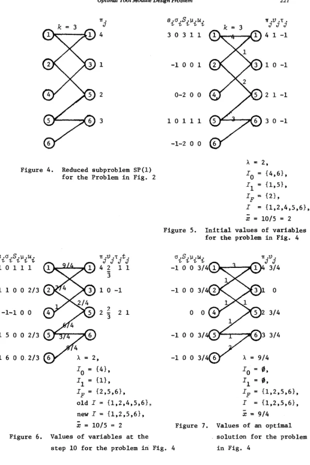
Consider the OTMP given in Figure 4. We will solve its relaxation problem by the algorithm D. The initial va]ueE of x ..

«i,j)

E

E),

A

1.-J

and other variables are decided by step 1 - 4 as shown in Figure 5. After several steps, the algorithm moves to step 10 and we show the values of variables and labells at that step in Figure 6. Since the

case 3 happens at the step 10, the set I becomes {1,2,5,6}. Next, the algorithm moves to the step 3 and

it

becomes

I

I

x .. /

III

=

(3+2+

i d

jEJ(i)

1.-J

2+2)/4

=

9/4. After several steps, the algorithm moves to the step 4 and the case that cr.

=

-1 for all

i

E I happens. He~e, we get an

1.-optimal solution shown in Figure 7 and the algorithm D terminates. In the remaining of this section it will be proved that the algo-rithm D is finite and the obtained solution (U,V,X,A,~) is an optimal solution of

(P)

and

(D).

Lemma 1. In the case of 1) or 3) at the step 10 in the algorithm D, the ~ E

M

which is in the old

I,

but not in the new

I

satisfie3

(5.1) - (5.12) for every

U

,j) E E in the fol1owing steps.

Proof:

Proof will be given for case 1). The case

3)

can be proved

similarly. By the labelling rules at step 4,5 and the changing rules of

x

ij

at step 6,7, every X~j (j E J(~» remains constant in the subsequent steps. Moreover, considering the step 9, u~ is always 0 in the sub-sequent steps. Hence, V. min

u.

u~ = 0 for any j E J(~).

1.-1f •

J

4

2

3

Figure 4. Reduced subprob1em SP(l) for the Problem in Fig. 2

s.cr.S.J,l.u.

1-1 0 1-1 1-1 1-1 1 1 0 0 2/3 -1-1 0 0 1 5 0 0 2/3 1f .V .T .t . J J J J 4 2 1 1

3

1 0 -1 2? 2 1

3

IO

= {4}, I1 = {l}, IF

=

{2,5,6}, old I

=

{1,2,4,5,6}, new I

=

{1,2,5,6},

x

=

10/5

=

2

Figure 6. Values of variables at the

s.cr.S.J,l.u.

1-3 0 1-311 -1 0 0 1 0-2 0 0 1 0 111 -1-2 0 0 1f .V .T • J J J 4 1 -1 1 0 -1 2 1 -1 3 0 -1 A

=

2,

IO

{4,6}, I1 {l,5}, IF = {2}, I

=

{1,2,4,5,6},

x

=

10/5

=

2

Figure 5. Initial values of variables for the problem in Fig. 4

cr.S.\.l.u.

1--1 0 0 3/4 -1 0 0 3/ 11 .V •

J J

3/4

A

=

9/4

IO

=

0,

I1

=

0,

3/4 IF = {l,2,5,6}, I

=

{1,2,5,6},

x

=

9/4

Figure 7. Values of an optimal

solution for the problem step 10 for the problem in Fig. 4 in Fig. 4

222 R. Hirabayashi, H. Suzuki and N. Tsuchiya

fore the complementarity (5.9) holds for every

(t,j)

E E. Also, it

could be easily verified that the other conditions (5.1) - (5.8) and (5.10) - (5.12) except (5.11) hold for t E M and j E

J(t)

in the

sub-sequent steps by taking account of the step 9.

Now, we show that the condition (5.11) holds for t E M in the

subsequent steps. In the step 10,

LX.

:>

.:e,

jEJ(i) iJ and (5.13)

L

x .. <:z,

jEJ(i) 1.-J

i

E

I (I

is the new

I),

holds. Moreover, the value of

I

x .

is fixed in the subsequent j EJ (i) i,7

steps. Since we assumed the case 1) and (5.13), A in the subsequent steps satisfies A <:

x

for the present value of

X.

Hence, in the any subsequent step, A >

I

xJ/" Since~.

=

max (0,

I

x.' - A)

=

0,

jEJ(i)

~ N jEJ(t) NJ

condition (5.11) holds.

0

Lemma

2. In the case of 2) or 4) on the step 10 in Algorithm D,

the suffix 2 E M which is in the old I, but not in the new I satisfies (5.1) - (5.12) for all (t,j) E

E

in the following step.

Proof: We prove it for case 2). The case 4) can be proved simi-larly. By the same reason mentioned in the proof of Lemma 1, every X

tj

(j E

J(t»

and

Ut

=

1 remain constant in the subsequent steps. Hence the conditions (5.1) - (5.12) except (5.9) always hold by considering the step 9.

Now, we show that condition (5.9) holds in the subsequent steps for every (t,j) E E.

J(t)

such that

Vj

< 1,

X

_tj

such that V j < 1 and xtj >

satisfies

u.O

= v.

< 1.

°

1, it suffices to show that for every j E

°

holds. Suppose there exists jo E

J(t)

0. Then, there exists a node

iO

E

M

which 1.-0 J

_a

(1) Suppose

iO

E

I

holds for the old

I.

Since the case 2) is assumed,

the node t is labelled (i.e. 0i ~ 0). Hence, by taking acount of x . >

tJ O

0, the node jo is labelled (i.e. T. ~ 0) by the labelling rule (step 5) J

_O

and the node

iO

is also labelled by the labelling rule (step 6). Hence, by assumeng the case 2),

I

x . .

<:

Z

> A holds and

u.

1 by

con-jEJ(i

O) 1.-oJ 1.-0

sidering the step 9. This is a contradiction.

(2) Suppose that

iO \

I fer the old I. Let l1S consider the preceding

step 10 at which

iO

is in the old

I,

but not in the new I at the pre-ceding step. Since

I

xi' <:

I

:r:.. holds, by taking acount of

jEJ(R.) J jEJ(i O) 1.-oJ

the reducing rule of the set I (step 10), i t is easily veri.fiE'd that the case 1) or 3) happens at the preceding step. Then we can easily show by the similar way to (1) that for every

i

c

I(jO)

n

I (I

is the new

I

at the preceding step 10), x .. = 0 holds. Hence, by the labelling rule

1.-J

O

(step 4 and 5), x ..

=

0

(i

E

I(jO)

n

I)

remains constant in the

sub-t.J 0

sequent steps. Therefore, X~j

=

0 holds and this is a contradiction.

0

Lemma 3.

When o. = -1 holds for any

i

E I at step 4, (5.1)

-

1.-(5.12) hold for every

(i,j)

E

E

at step 9 and Algorithm D stops.

Proof:

By Lemma 1 and 2, it is sufficient to show that the

comple-mentarity (5.9) holds for any

(i,j)

E

E

where

i

E

I.

If

S.

> 0 for some

1.-i

E

I

the cri

=

O. Then, by the assumption of Lemma 3,

Si

0 for every

i

E

I.

Hence,

LX.. -

x

=

S -:

= 0 and

u -:

= (k -

I

Il

U

{i

E

M

I

i

Is.

I

jEJ(i)

1.-J v v

and

_ui

1}1) /

IIFI

for every

i

E

I.

SUPPoEe there exists an

iO

E

I

and a jo E

J(i

O

)

such that the complementarity (5.9) does not hold. Since

v.

=

min

u.

< U.

, x . .

> 0 and V.

=

0 hold, then we can

J O

iEI(jO)

1.- 1.-0 1.-rflo J O

derive a contradiction in the same way to prove the Lemma 2. 0

Theorem

3. Algorithm D stops in the finite steps and gives optimal

solutions for

(P)

and

(D).

Proof:

At first, we will prove that the node set I will decrease

monotonously at the step 10. If

L

x ..

=;;

holds for every i E I,

jEJ

(0

1-J

then the case that cr.

=

-1 for all i E I happens at the step 4 and

1.-Algorithm D does not move to the step 10. I such that

Lx..

> ;; >

LX.. .

Hence, there exis ts i 0 ,i 1 E Then, by step 3 - step 8,

jEJ (i

o) 1.-07

jEJ (i

1) 1.-~:J

cr. 0 and cr.

=

-1 hold. Suppose the case 1) or 3) occurs, i

l Is. I

h~2ds

for

the1.-~ew

I . Suppose the case 2) or 4) occurs,

iO

!i I for the

new I. In any case, the set I is monotone decreasing.

Furthermore, when

I

decreases monotonously, for all elements i E

M

leaving

I,

conditions (5.1) - (5.12) hold in the subsequent steps by Lemma 1 and 2. Suppose

III

1 then assumption of Lemma 3 holds by considering the step 3 and 4. Hence, in the algorithm D, the assumption of Lemma 3 holds at some step and conditions (5.1) - (5.12) hold for every

(i,j)

E

E

by Lemma 3. Therefore, the algorithm stops in the finite steps and the solution (u 'v 'x ,A. ,J1) obtained gives optimal solu-tions for (P) and (D). 0

224 R. Hirabayashi, H. Suzuki and N. Tsuchiya

6. Numerical Examples and Computational Experiences

Consider the OTMP given by Table 1 where the maximum size of tool magazine is

k

=

8. We will solve it and get an optimal solution as shown in the following.

u

= (1,0,1,1,1,0,1,0,0,1,1,0,0,1,0), V

(1,0,1,0,0,1,0,0,0,0,1,0,0,0,0,0,0,0,1,1,0,1,0,0,0) or the tool module

U

=

{1,3,4,5,7,10,11,14} and the parts family

V

=

{j E

N

I

I(j)

c

U}

=

{l,3,6,1l,19,20,22} is an optimal solution for the problem. This solu-tion is obtained by executing the branch and bound algorithm for 49 nodes and the CPU time is 0.88 seconds by Hitac M-180.

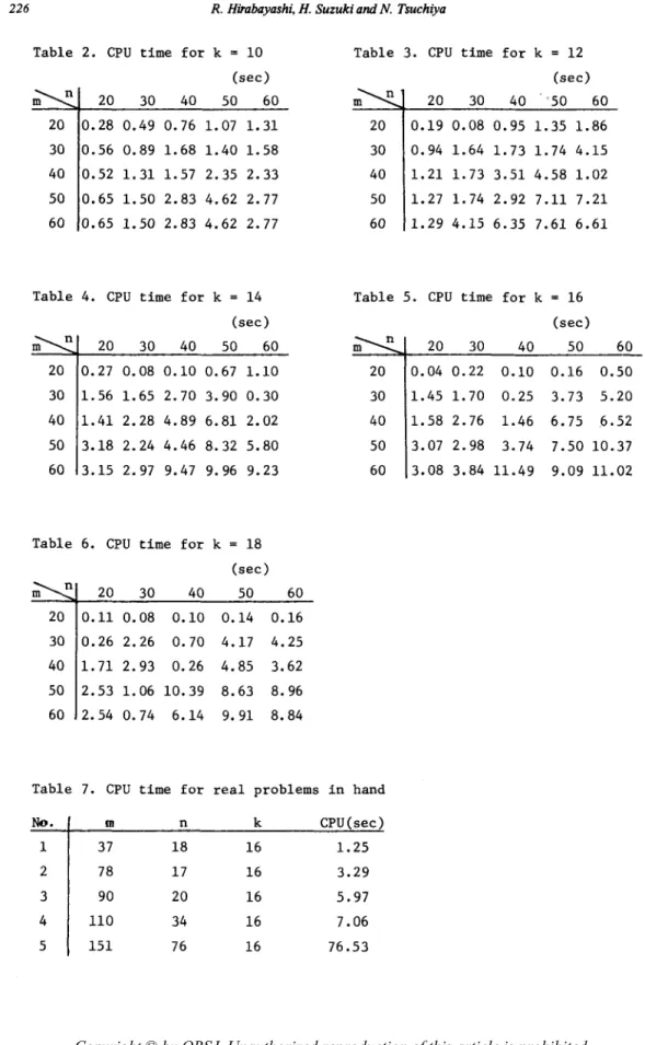
The other computational examples are shown in Tables 2 - 7. There, for the same size of

m

and

n,

the structures of problems (i.e. the set

E

and TI) are the same and only k varies. The structures of the problems are chosen from the real OTMP's available. Some real OTMP's are shown in Table 7. By these examples, we verified that the algorithm we pro-posed is quite efficient and can solve practical problems.

7. Concluding Remarks

Among the set-up operations hindering the improvement of produc-tivity of NC machines and their unmanned operations, the tool changing operation is essential and unavoidable. To reduce the frequency of set-up operations for the tool changing operation,

tool module

method has been proposed. However, the problem of designing an optimal tool module is unsolved. In this paper, we have pointed out that for this

tool

module

method, there are two mathematical programming problems, i.e.,

(1) Optimal Parts Grouping Problem, (2) Optimal Tool Module Design Problem.

Here, we have proposed for the latter problem a method which is a combi-nation of a branch and bound method and a network flow method. More-over, we have verified through numerical examples that the proposed method is quite efficient.

Also, we have pointed out that the latter problem includes some practical problems such as a problem to find the tool module maximizing the number of processing parts or a problem to find a tool module making possible the longest time unmanned operation of a factory with no tool change. We can further point out that the latter problem is regarded as a subproblem for the former one. By the column generation approach, the OPGP can be formulated as a set covering problem described as follows.

'"

'"

E ~ .c>

~

.~

~

~

oS

~

~

I

~

X

1 1 1 2 3 4 1 5 6 7 1 8 9 10 11 1 12 13 14 15 1\". 1 .1 2 3 4 5 6 7 1 1 1 1 1 1 1 1 1 1 1 1 1 1 1 1 1 1 1 1 1 1 1 1 1 1 1 1 1 (kz₈₎ 8 9 10 11 12 13 14 15 16 17 18 19 20 21 22 23 24 25 1 1 1 1 1 1 1 1 1 1 1 1 1 1 1 1 1 1 1 1 1 1 1 1 1 1 1 1 1 1 1 1 1 1 1 1 1 1 1 1 1 1 1 1 1 1 1 1 1 1 1 1 1 1 1 1 1 1 1 1 1 1 1 1 1 1 1 1 1 1 1 1 1 1 1 1 1 1 1 1 1 1 1 1

226 R. Hirabayashi, H. Suzuki and N. Tsuchiya

Table 2. CPU time for k

=

10 Table 3. CPU time for k

=

12

(sec) (sec) n _{20 30 40 50 60 20 30 40} 50 60 m 20 0.28 0.49 0.76 1. 07 1. 31 20 0.19 0.08 0.95 1.35 1.86 30 0.56 0.89 1. 68 1.40 1. 58 30 0.94 1.64 1. 73 1. 74 4.15 40 0.52 1. 31 1. 57 2.35 2.33 40 1. 21 1. 73 3.51 4.58 1.02 50 0.65 1. 50 2.83 4.62 2.77 50 1.27 1. 74 2.92 7.11 7.21 60 0.65 1.50 2.83 4.62 2.77 60 1.29 4.15 6.35 7.61 6.61

Table 4. CPU time for k

=

14 Table 5. CPU time for k

=

16

(sec) (sec) n 20 30 40 50 60 n 20 30 40 50 60 m m 20 0.27 0.08 0.10 0.67 1.10 20 0.04 0.22 0.10 0.16 0.50 30 1.56 1. 65 2.70 3.90 0.30 30 1.45 1. 70 0.25 3.73 5.20 40 1.41 2.28 4.89 6.81 2.02 40 1.58 2.76 1.46 6.75 .6.52 50 3.18 2.24 4.46 8.32 5.80 50 3.07 2.98 3.74 7.50 10.37 60 3.15 2.97 9.47 9.96 9.23 60 3.08 3.84 11.49 9.09 11.02

Table 6. CPU time for k

=

18 (sec) n ₂₀ 30 40 50 60 m 20 0.11 0.08 0.10 0.14 0.16 30 0.26 2.26 0.70 4.17 4.25 40 1. 71 2.93 0.26 4.85 3.62 50 2.53 1. 06 10.39 8.63 8.96 60 2.54 0.74 6.14 9.91 8.84

Table 7. CPU time for real problems in hand

No. m n k CPU (sec)

1 37 18 16 1.25

2 78 17 16 3.29

3 90 20 16 5.97

4 110 34 16 7.06

Enumerate all tool combinations for a given set of tools

i

1,2,···,m. Since tools in a module must be within ~he maximum size k of tool magazine, the total number of modules is T

=

L et

and we denote

t-lm

each tool module by t

=

1,2,···,T. Denote by the m=aimensional 0-1 vector

u(t)

=

(u (t) u (t) ••• u

(t»T the t-th tool module and by

n

1 ' 2 ' , dimensional 0-1 vector

vet) =(v

l

(B)

,v

2

(t) , •••

,v

(t»T the set of parts

(t) (t) n

that can be processed by

u

,

where

u.

=

1 (= 0) means the tool

~

(t)

module t includes (does not include) the tool i and

v.

=

1 (= 0)

J

means that it is (not) possible to process part j by the tool module t. Then, the OPGP is formulated as the well-known set covering problem:

T (Q) minimize

L

Y t t=l subject to T (t)

LV

Y

_t

~e, t=l Y

_t

E {O,U,

t

1,2,···,T,

where e is an m-dimensional vector (l,l,···,l)T, and

Yt

= 1 (= 0) means that the optimal set of tool modules contains (does not contain) the t-th tool module

u(t).

One of the difficulties of this approach is that it takes a lot of time to generate all tool modules

u(t)

and the corres-ponding part sets

vet)

respectively.

Now, suppose some of coefficient column vectors (1. e., parts fami-lies) are known for (Q) such that every part belongs to at least one of these known parts-families, and we call this problem by (R). Denote by

(R)

the LP relaxation problem of (R). By solving

(R),

the dual optimal solutions IT. (j = 1,2,··· ,n) is obtained corresponding to each

const-J

raint. Since lT

j is a shadow price. for the constraint j (Le., the part j), it can be considered that IT. shows a value to process the part j. In this sense, the problem to find a most valuable parts family

vet)

and the corresponding tool module

u(t)

is:

(P) maximize

L

IT.V. jEN J J subject to V j $

u

_{i '}

LU.$k,

iEM

~ (i,j) E E,

228 R. Hirabayashi, H. Suzuki and N. Tsuchiya u. € {O,l}, 1.-V. € {O,ll, J

i

€

M,

j €

N.

This is evidently the OTMP disscussed in this paper.

Now, it is possible to develop an effective method for solving

(Q).

By solving (P), we obtain its optimal solution

u*, v*

where

V*

represents the parts that can be processed by

u*.

After that, we add

v*

to (R) as a new column vector

v(t).

Thus, we can generate only meaningful columns of

(Q),

which are possibly needed to construct an optimal solution for

(Q),

and it will be enough to solve the set covering problem with smaller size instead of

(Q).

Acknowledgment

The authors wish to thank the editor and reviewers for their helpful comments in revising the paper.

References

[1] Geoffrion, A. M.: Lagrangean Relaxation for Integer Programming,

Mathematical PrgPamming Study,

Vo1.2 (1974), 82-114.

[2] Kobayashi, T.: The Lexico-Shortest Route Algorithm for Solving the Minimum Cost Flow Problem with an Additional Linear Constraint.

Journal of the Operations Research Society of Japan,

Vo1.26, No.3

(1983), 167-185.

[3] Kobayashi, T.: The Lexico-Bounded Flow Algorithm for Solving the Minimum Cost Project Scheduling Problem with an Additional Linear Constraint.

Research Report

B-82-4, Saitama University

(August, 1982).

[4] Law1er, E.L.:

Combinatorial Optimization: Networks and Matroids.

Halt, Rinehart and Winston, New York, 1976.

[5] Tanaka, N., Tsuchiya, N. and et. al.: A Study in Parts Classifi-cation by Used Tools (in Japanese).

Proceeding of spring Conference

of Japan Industrial Management Association,

1982, 129-130.

Ryuichi HIRABAYASHI: Department of Industrial Engineering, Tokyo Science University, Kagurazaka 1-3, Shinjllku-ku, Tokyo, 162, Japan.