On the number of reduced trees, cographs, and series-parallel graphs by compression

全文

(1)Vol.2011-AL-137 No.6 2011/11/18 IPSJ SIG Technical Report. 1. Introduction. On the number of reduced trees, cographs, and series-parallel graphs by compression Takeaki Uno ,†1 Ryuhei Uehara and Shin-ichi Nakano †3. Tree is one of basic models frequently used in various areas including searching for keys, modeling computation, and parsing a program. Since an explicit storage of a tree of a large size needs huge amount of memory, a compact representation is desired. A typical example is a trie structure that compresses a given huge word dictionary by taking the prefixes of words 12) [Chapter 6.3]. In the area of data mining, the other basic models are also used to represent a tons of data having some specific structure. In this context, there are a lot of papers for encoding trees, plane graphs, plane triangulations. For example, see 8), 10), 14) for trees, 5), 11) for plane graphs, and 1), 16) for maximal plane graphs, and referred papers. In this paper, we first focus on the “unordered reduced” trees, in which the children of each vertex has no ordering and no vertex has exactly one child. The unordered reduced tree is one of important models from both theory and practice. We first give an efficient representation of an unordered reduced tree. The representation requires 2` − 2 bits to represent a given unordered reduced tree with ` ≥ 2 leaves, whereas a known folklore representation uses a bit string of length 2n − 2 which is a representation of an ordered tree with n vertices. Note that ` ≤ n < 2` holds for any unordered reduced tree. Computation of the representation can be done efficiently; both of encoding and decoding can be done in O(`) time. To the best of our knowledge this is the first non-trivial compact representation designed for unordered reduced trees. It is worth mentioning that we do not use the big-O notation. Hence the length of the representation gives us an upper bound of the number of unordered reduced trees with ` ≥ 2 leaves; the number of unordered reduced trees with ` ≥ 2 leaves bounded by 22`−2 . We here compare our results with the notion of succinct representations of trees7),8),10),13),14) . A succinct representation for a class of some structure is a way to map each member of the class to a sufficiently short bit string. The best representation for trees needs only 2n+o(n) bits, and it also supports a rich set of queries in O(1) time for each. On the other hand, since the information-theoretic lower bound to represent an “ordered” tree having n node is 2n − O(log n)8) , the representation is optimal in a sense. However, such a framework has two flaws. †2. We give an efficient encoding and decoding scheme for computing a compact representation of a graph in one of unordered reduced trees, cographs, and series-parallel graphs. The unordered reduced trees are rooted trees in which (i) the ordering of children of each vertex does not matter, and (ii) no vertex has exactly one children. This is one of basic models frequently used in many areas. Our algorithm computes a bit string of length 2`−1 for a given unordered reduced tree with ` ≥ 1 leaves in O(`) time, whereas a known folklore algorithm computes a bit string of length 2n − 2 for an ordered tree with n vertices. Note that in an unordered reduced tree ` ≤ n < 2` holds. To the best of our knowledge this is the first such a compact representation for unordered reduced trees. From the theoretical point of view, the length of the representation gives us an upper bound of the number of unordered reduced trees with ` leaves. Precisely, the number of unordered reduced trees with ` leaves is at most 22`−2 for ` ≥ 2. Moreover, the encoding and decoding can be done in linear time. Therefore, from the practical point of view, our representation is also useful to store a lot of unordered reduced trees efficiently. We also apply the scheme for computing a compact representation to cographs and series-parallel graphs. We show that each of cographs with n vertices has a compact representation in 2n − 1 bits, and the number of cographs with n vertices is at most 22n−1 . The resulting number is close to the number of cographs with n vertices obtained by the enumeration for small n that approximates Cdn /n3/2 , where C = 0.4126 · · · and d = 3.5608 · · · . Series-parallel graphs are well investigated in the context of the graphs of bounded treewidth. We give a method to represent a seriesparallel graph with m edges in d2.528m − 2e bits. Hence the number of seriesparallel graphs with m edges is at most 2d2.528m−2e . As far as the authors know, this is the first non-trivial result about the number of series-parallel graphs. The encoding and decoding of the cographs and series-parallel graphs also can be done in linear time.. †1 国立情報学研究所 (National Institute of Informatics) †2 北陸先端科学技術大学院大学 (Japan Advanced Institute of Science and Technology) †3 群馬大学 (Gunma University). 1. c 2011 Information Processing Society of Japan.

(2) Vol.2011-AL-137 No.6 2011/11/18 IPSJ SIG Technical Report. with m edges is at most 2d0.528me . The encoding and decoding of the seriesparallel graphs also can be done in linear time.. from the practical point of view. First, the factor of o(n) is hard to determine a priori. That is, when we execute the algorithm, we may have to perform memory allocation process dynamically that spoils efficiency. Second, the hidden constant factor in o(n) becomes huge in general. Hence, some succinct representation is not practical for small n. Also, this framework is not applicable to estimate the number of members in the class. We next apply the compact representation of unordered reduced tree to the other graph classes; cographs and series-parallel graphs. For the last decade, many graph classes have been introduced3) . Among them, cographs form one of basic graph classes. Since they have a simple recursive structure, the class is a subset of many important graph classes, and hence some intractable problems on general graphs become tractable on cographs. The simple recursive structure of a cograph can be represented by a canonical unordered reduced tree. Hence we can estimate that the number of cographs with n vertices is at most 22n−1 . In the context of the implicit representation of the graph class, it is mentioned that the number of cographs is 2O(n log n) 15) [Sect. 8.1]. We exponentially improve this upper bound, and we again mention that we do not use the big-O notation. According to The On-Line Encyclopedia of Integer Sequences (http://oeis.org/A000084), the number of cographs with n vertices is estimated as Cdn /n3/2 , where C = 0.4126 · · · and d = 3.5608 · · · . This value is obtained by the enumeration for small n, and our upper bound is close to this estimation. The encoding to a bit string from a given cograph and the decoding of the bit string to the original cograph can be done in linear time. The other graph class is series-parallel graphs. This is also one of basic graph classes, and this class is well investigated in the context of the graphs of bounded treewidth. However, recently, it is revealed that many data obtained from the bioinformatics area can be modeled in this graph class. For example, the E.coli metabolic network has treewidth 3 and more than 90% of pathways of several organisms are series-parallel graphs4) . Therefore, the importance of this class increases more and more. As far as the authors know, there are no known nontrivial results about the compact representation designed for the class and the number of series-parallel graphs. We give a method to represent a series-parallel graph with m edges in d0.528me bits. Hence the number of series-parallel graphs. 2. Preliminaries Let G be a graph. The degree of a vertex in G is the number of vertices adjacent to the vertex. A tree is a connected graph with no cycle. A rooted tree is a tree in which one vertex r is designated as the root. For each vertex v in a tree, let P (v) be the unique path from v to r. The parent of v 6= r is the unique vertex in P (v) adjacent to v, and the ancestors of v are the vertices in P (v). The parent of r is not defined. The only ancestor of r is r itself. We say if v is the parent of u then u is a child of v, and if v is an ancestor of u then u is a descendant of v. Note that each vertex v is always a descendant of v. The height of a vertex v is the number of edges on the longest path from v to a descendant of v. A leaf is a vertex having no child. The height of a leaf is always 0, and the height of a vertex is always larger than the height of its child. In particular, the height of a vertex is the maximum height of its children plus one. A reduced tree is a rooted tree in which no vertex has exactly one child. In2) a reduced rooted tree is called a homeomorphically-irreducible rooted tree. Note that the root of a reduced tree may have degree two, although no vertex has degree two in a similar graph called a reduced non-rooted tree, which is a non-rooted tree with no vertex of degree two. A rooted tree is an ordered tree if the children of each vertex are linearly ordered, and an unordered tree otherwise. A full-binary tree is an ordered (rooted) tree in which each vertex has zero or two children. If vertex v has the ordered children (vL , vR ), vL is called the left child and vR is called the right child of v. A path (v1 , v2 , · · · , vj ) in a full-binary tree, satisfying that each vi is the left child of vi+1 for i = 1, 2, · · · , j − 1, is called a left-down path. A left-down path is maximal if it is not a proper subpath of any other left-down path. A left-down path from a vertex v to its ancestor u is denoted by the sequence of its vertices starting from v and ending with u. 3. Compact Representation of Unordered Reduced Trees In this section, we assume that the input is an unordered reduced (rooted) tree T with ` leaves. See an example in Fig. 1(a).. 2. c 2011 Information Processing Society of Japan.

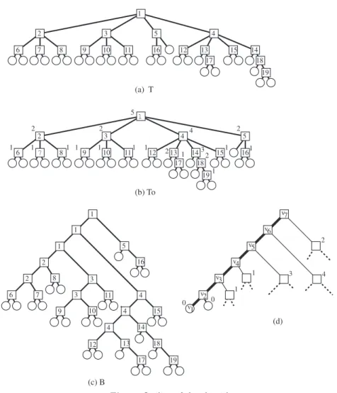
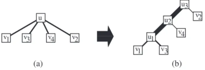
(3) Vol.2011-AL-137 No.6 2011/11/18 IPSJ SIG Technical Report. k − 1 (Fig. 2), the ordered reduced tree TO is transformed into a full-binary tree B. See Fig. 1(c). Note that both TO and B still have ` leaves. Finally, B is encoded into a bit string S of length 2` − 1. The encoding of B is done by a depth first tree traversal, in which each edge is traversed exactly twice in opposite direction. When an edge is traversed downward, a “0” is appended to bitstring S, and when an edge is traversed upward, a “1” is appended to S. From the bitstring S one can easily reconstruct BI and then B. However, to reconstruct TO from B, we need to divide each maximal left-down path of B into left-down subpaths so that each subpath corresponds to a vertex in T . Thanks to the linear ordering of children, we can always uniquely divide each left-down path of B into suitable left-down subpaths. By ignoring the linear ordering of children, T is derived from TO . 3.1 Encoding an unordered reduced tree Now we give an encoding algorithm for unordered reduced trees. We begin with a linear ordering of children, which is the key to our compact representation. Let T be an unordered reduced tree with ` leaves. Let (v1 , v2 , · · · , vk ) be the sequence of children of a vertex u. We assume the heights of the vertices are increasing order in the sequence, i.e., v1 has the smallest height and vk has the largest height. The linear ordering of children is the sequence obtained by removing v2 from the sequence and append v2 to the last, that is, (v1 , v3 , v4 , · · · , vk , v2 ). Note that each non-leaf vertex always has two or more children, thereby the sequence above is always defined. The linear orderings define an ordered reduced tree TO obtained from T . See Fig. 1(b). Intuitively, among the children of each vertex, the leftmost child has the minimum height, the rightmost child has the second minimum height, and the rest of children appear between them with increasing order of heights. Our idea of a compact representation is to represent TO by a full-binary tree with the same number of leaves. We replace each non-leaf vertex u of T having k > 0 children by a left-down path of length k − 1 as shown in Fig. 2. We call the left-down path the expand path of u, and denote it by L(u). In the replacement, we keep the linear ordering of the children. When the linear ordering of children of u is (v1 , . . . , vk ) and L(u) = (u1 , . . . , uk−1 ), we set v1 to the left child of u1 , v2 to the right child of u1 , v3 to the right child of u2 , . . ., vi to the right child. 1 2 6. 3. 7. 8. 9. 5. 10. 11. 4. 16. 12. 13 17. 15. 14 18 19. (a) T 5 2 2 1. 1. 6. 1. 2 3 8. 7. 1 1. 1. 9. 4. 10. 11. 1. 1. 12. 2. 4. 5. 2 13 1 14 3 2 17 18 19. 15. 1. 16. 1. 1. (b) To v7. 1 v6. 1. 8. 2 6. v4. 16. 2. 3 10. 4. 15. 3. 4. 1. v1. (d). 14. 4 12. v2 0. 4. 11. 0 9. 1. v3. 3. 7. 2. v5. 5. 1. 18. 13 17. 19. (c) B. Fig. 1 Outline of the algorithm. The outline of our algorithm is as follows. We first give a linear ordering of children of each vertex of T by a simple rule. Now the unordered reduced tree T is transformed into an “ordered” reduced tree TO (Fig. 1(b)). Then, by replacing each non-leaf vertex of TO having k > 0 children by a left-down path of length 3. c 2011 Information Processing Society of Japan.

(4) Vol.2011-AL-137 No.6 2011/11/18 IPSJ SIG Technical Report. S = 111111001001001110010010011110010100101010010010100. We can see that one can reconstruct B from the bit string S by simulating the traverse. In the next section, we will show that the expand path of each vertex can be extracted from the maximal left-down paths thanks to the linear ordering, therefore the reconstruction of the original unordered reduced tree T from the bit string S can be done uniquely and efficiently. We have the following theorem. Theorem 1 One can compute in O(`) time a bit string of length 2` − 1 representing an unordered reduced tree with ` leaves. 3.2 Decoding an unordered reduced tree It is clear that the full-binary tree B can be obtained from the bit string S. Since T is an unordered tree, it is enough to show that TO can be reconstructed from B. The purpose of this section is to establish a way to extract expand paths of all vertices in TO . We choose a maximal left-down path and extract all the expand paths included in the path. We start from the rightmost maximal left-down path, and iteratively process maximal left-down paths from right to left. Therefore, when we process a left-down path L, the extraction has been done in descendants of the right child u of any vertex in L. See an example in Fig. 1(d). This implies that we have constructed all the subtrees of TO rooted at the descendants of u, and hence we can compute the height of any child x of a vertex vi in the left-down path L. Set h(vi ) be the height of the right child of vi . The extraction of expand paths is done in a bottom up way. Suppose that L = (v1 , . . . , vk ). We first observe that v1 itself corresponds to a leaf of TO , thus the lowest expand path L(x) starts from v2 . We find the other end vj of L(x) by looking at the heights of right children of v2 , . . . , vk one by one, so that cutting L at the vertex will not result the violation of the linear ordering. In precise, vj is the vertex in the ancestor of v2 whose right child has the smallest height among the right children of all ancestors of v2 . Then the next lowest expand path starts from vj+1 , and in the same way we can find the other end. In this way, we iteratively extract the expand paths until we reach to the top of L. The upside end vertex of an expand path is characterized by the following lemma. This is the key to the extraction of expand paths. Lemma 2 Suppose that an expand path L(u) in T) is (vi , . . . , vj ) for some vj .. u3 u v1. v3. u2 v4. vv4. u1. v2 v1. (a). vv2. v3. (b). Fig. 2 Replace a vertex v by a left-down path. of ui−1 , . . ., and vk to the right child of uk−1 . For a rooted ordered tree T in Fig. 1(a), the resulting full-binary tree B is drawn in Fig. 1(c). Essentially, our compact representation is a bit string representing B. The algorithm to compute the representation is as follows. Algorithm (T : an unordered reduced tree) 1. compute the height of each vertex in T ; 2. sort the children of each vertex by their heights; 3. compute the linear ordering of the children of each vertex; 4. replace each node having more than two children by the left-down path with keeping the linear ordering of children; 5. remove all leaves from the resulting tree B; 6. output the bit string representing B (by the depth first tree traversal). The height of each vertex of T can be computed in O(`) time in a bottom up way. The sorting of the children can be done in O(`) time, by processing all sortings at once by bucket sort. We here describe the details of step 6 that encodes the resulting tree B. We put a label 0 to each leaf and 1 to inner nodes. We then compute the pre-order of vertices by a depth-first search going left child first, and right child next. The pre-order is the visiting order by the depth-first search; at the beginning of the search, the sequence is empty, and when a new vertex is visited by the search, the vertex is added to the end of the sequence. The bit string is the sequence of vertex labels ordered by the pre-order. For example, the tree T in Fig. 1(a) is encoded to. 4. c 2011 Information Processing Society of Japan.

(5) Vol.2011-AL-137 No.6 2011/11/18 IPSJ SIG Technical Report. Then, vj is the uppermost vertex in the maximal left down path L including L(u) such that h(vj ) ≤ h(vi ). Proof.Let vl is the uppermost vertex in L such that h(vl ) ≤ h(vi ). We will prove that vl = vj . Note that vl can be vi , and vj can be vi . Suppose that vl is a proper descendant of vj , i.e., vl ∈ L(u) and vl 6= vj . Then, u has at least three children, and the heights of children are h0 , h(vj ), . . . , h(vl ), where h0 is the height of the first child of u. From the definition of vl , h(vl ) < h(vj ), however this contradicts to the linear ordering. Therefore, vl is not a proper descendant of vj . We next suppose that vl is a proper ancestor of vj , i.e., vl 6∈ L(u). Let L(u0 ) = (vi0 , ..., vj 0 ) be the expand path of u0 which includes vl . Observe that the height of the left child w of u0 is no less than the height of u since w is an ancestor of u. This implies that h(vl ) is smaller than the height of w, since the height of u is strictly larger than h(vi ). This contradicts to the linear ordering. From these, we conclude that vl = vj . Lemma 2 claims that the highest vertex vl in L s.t. h(vl ) ≤ h(vi ) is the other end vertex of L(u). Such a vertex vl can be found by looking the heights of all vertices in L, thus we obtain the following algorithm to reconstruct T from S.. A naive implementation makes this algorithm run in O(|S|2 ) time, where |S| is the length of the bit string S. We explain how to compute it in O(|S|) time. Let L = (v1 , . . . , vk ) be a left-down path and L(u) = (vi , . . . , vl ) be an expand path included in L. We suppose that vi 6= vk , otherwise vl = vi . Let vj , j > i be the lowest vertex satisfying h(vj−1 ) > h(vj ). If there is no such vertex, vj is not defined. vj 0 is the highest vertex satisfying h(vj 0 ) = h(vi ). Note that vi can be vj 0 , and vj 0 is always defined. The key observation is that in the linear ordering, children on the middle are sorted in the increasing order of their heights. From the observation, we have the following lemma. Lemma 3 (1) vl = vj holds if vj is defined and h(vj ) < h(vi ), and (2) vl = vj 0 holds if h(vj ) ≥ h(vi ) or vj is not defined. Proof.We first observe that vl never be a proper ancestor of vj , from the linear ordering. Similarly, if vj is defined, no ancestor of vj has a height smaller than or equal to vi ; otherwise the linear ordering contains a decreasing point at the middle. This together with the definition of vl implies that if vj is defined and h(vj ) < h(vi ), vl = vj holds. If vj is defined but h(vj ) ≥ h(vi ), we have vl = vj 0 . In the case that vj is not defined, heights of the vertices in (vi , vi+1 , · · · , vk ) are monotonically non-decreasing, thus the highest vertex having the height no more than vi is vj 0 . This implies vl = vj 0 , and we conclude the lemma. From Lemma 3, the task to find an expand path is to find both vj and vj 0 . This can be done in O(j − i) time as follows: If vl = vj , then we never access to the vertices {vi , . . . , vj }. If vl = vj 0 , we set vi to vj 0 +1 , and find vj and vj 0 again to find the next expand path. However, in this case, we know that even for new vi , the previous vj is still the lowest vertex satisfying h(vj−1 ) > h(vj ). Thus, we do not need to compute vj again. In summary, each vertex in a maximal leftdown path is accessed twice; once for finding vj and once for finding vj 0 . Here, the algorithm maintains two lists. The first list consists of the vertices vj with h(vj−1 ) > h(vj ) from descendants, and the second list consists of the vertices of the same height. Both lists can be maintained in linear time, and they admit us to find vj and vj 0 in O(1) time. Thus, the extraction of expand paths from a maximal left-down path L can be done in O(|L|) time. Therefore, any bit string that represents an unordered reduced tree can be. Algorithm Decode (S: bit string) 1. B := the full-binary tree obtained from S 2. V := ∅ 3. for each maximal left down path L from right to left 4. remove the leaf v from L, and V := V ∪ {v} 5. compute the height of each vertex in L 6. while L is not empty 7. vi := the lowest vertex in L 8. vl := the highest vertex such that h(vl ) ≤ h(vi ) 9. remove the subpath from vi to vl , and insert it to V 10. end while 11. end for 12. E := edge set induced by the parent-child relation of expand paths and leaves in B. 5. c 2011 Information Processing Society of Japan.

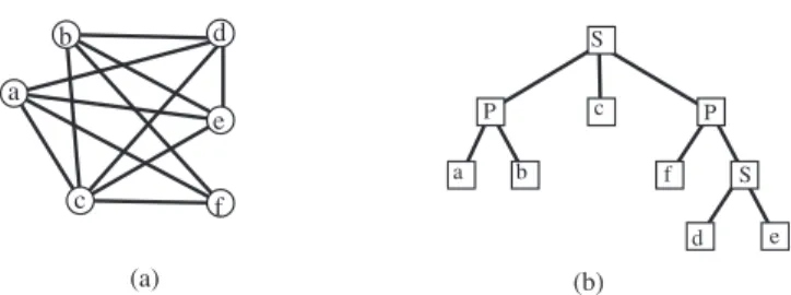
(6) Vol.2011-AL-137 No.6 2011/11/18 IPSJ SIG Technical Report. decoded uniquely. Thus no two different unordered reduced trees are encoded into the same bit string. Hence we have the following theorems. Theorem 4 For any ` ≥ 1, there is a 1-to-1 mapping from the set of unordered reduced trees of ` leaves to the set of bit strings of length at most 2` − 1. Theorem 5 From a bit string of length 2` − 1 representing an unordered reduced tree with ` ≥ 1 leaves, the tree can be reconstructed in O(`) time. Since the first bit of the bit string is always 1 when the original unordered tree has at least two leaves, we obtain the following theorem. Theorem 6 The number of unordered reduced trees with ` ≥ 1 leaves is at most 22`−2 .. d. b. S. a a. c. c. P. e. b. P f. S. f d. (a). e. (b). Fig. 3 A cograph and its canonical tree representation. It is known that the canonical tree representation of a cograph can be obtained in O(n+m) time, where n is the number of vertices and m is the number of edges in the cograph. From the canonical tree representation one can reconstruct the original cograph in O(n + m) time. We have the following theorem. Theorem 8 One can compute in O(n + m) time a bit string of length 22n−1 representing a cograph with n vertices and m edges. One can also construct the cograph from the bit string in O(n + m) time.. 4. Compact Representation of Cographs Let G1 = (V1 , E1 ) and G2 = (V2 , E2 ) be two arbitrary disjoint graphs. A graph G = (V, E) is the parallel composition of G1 and G2 if V = V1 ∪ V2 and E = E1 ∪ E2 . A graph G = (V, E) is the series composition of G1 and G2 if V = V1 ∪ V2 and E = E1 ∪ E2 ∪ {(x1 , x2 )|x1 ∈ V1 , x2 ∈ V2 }. A cograph is a graph composed of one vertex, or a graph obtained from two cographs with these two operations. It is well known that any cograph has a canonical tree representation6),9) , in which (1) each leaf corresponds to each vertex of the graph, (2) each internal vertex has a label corresponding to either a series or parallel composition, and (3) on every path in the tree, the labels appear alternatively. We note that (1) implies that the number of leaves of the tree is n for any cograph of n vertices. Each such canonical tree corresponds to a unique cograph up to isomorphism, thus no two cographs are made from the same canonical tree and vice versa. Fig. 3 shows an example of a cograph and its canonical tree representation. Each non-leaf vertex has at least two children and the ordering of them does not matter, so the tree structure is an unordered reduced tree. Thus an unordered reduced tree corresponds to two cographs; one with the root label of the series composition, and the other with the root label of the parallel composition. Hence the number of cographs of n vertices is twice of the number of unordered reduced trees of n leaves which is equal to 22n−2 . Therefore, the following theorem holds: Theorem 7 The number of cographs with n vertices is at most 22n−1 .. 5. Compact Representation of Series-Parallel Graphs Let G = (V, E, s, t) be a multi graph with two designated vertices s and t, called the terminals. A multi graph is a graph that can contain two or more identical edges having the same endpoints. A graph G = (V, E, s, t) is the parallel composition of G1 = (V1 , E1 , s1 , t1 ) and G2 = (V2 , E2 , s2 , t2 ) if V = V1 ∪ V2 and E = E1 ∪ E2 and s = s1 = s2 and t = t1 = t2 . A graph G = (V, E, s, t) is the series composition of G1 = (V1 , E1 , s1 , t1 ) and G2 = (V2 , E2 , s2 , t2 ) if V = V1 ∪ V2 and E = E1 ∪ E2 and s = s1 , t1 = s2 , t2 = t. The series and the parallel composition can easily be generalized to more than two graphs. A graph G = (V, E, s, t) is a series-parallel graph with terminals s and t if it consists of only one edge {s, t} or it results from the applications of the series or the parallel compositions to two or more series-parallel graphs. It is well known that any series-parallel graph has a tree structure which describes how the graph is composed3) , and no two series-parallel graphs with two terminals are generated from the same tree structure. Similar to cographs, the structure is a reduced tree with alternative labels, but the difference is that the. 6. c 2011 Information Processing Society of Japan.

(7) Vol.2011-AL-137 No.6 2011/11/18 IPSJ SIG Technical Report. that u is a leaf implies that x is a series composition. From the above observation, we can determine the label of x 6= z whose expand path is included in L, by looking at the right children of the vertices in the path. Thus, we cannot get the label of L(z) only when L(z) is the unique expand path in L. In this case, we have to memory the label of z by using additional bits. Let U (L) = (u1 , . . . , uk0 ) be the vertices in L such that their right children are leaves. We have to distinguish the following (k 0 + 1) cases. 1 : u1 , u2 , . . . , uk0 ∈ L(z) and their labels are “Series” 2 : u1 ∈ L(z) and its label is “Parallel” 3 : u1 , u2 ∈ L(z) and their labels are “Parallel” ... 0 k : u1 , u2 , . . . , uk0 −1 ∈ L(z) and their labels are “Parallel” k 0 + 1 : u1 , u2 , . . . , uk0 ∈ L(z) and their labels are “Parallel” Note that, in the case 2 to k 0 + 1, we can determine that all labels of the other vertices in U (L) are “Series.” We put the index of the corresponding case to each left-down maximal path, and this information is sufficient to reconstruct T and know the labels of the vertices. The maximum ∏bits to store the information is equal to (|S| + 1) | P is a partition of {1, . . . , n}}. log2 max{. a. a. multiply. a. h h g. a. h. d. multiply. path. f. a. path. e. d. path. d. b. e. h g. f a e j. j. h i. g. j multiply. b. f. a e b. d j. d. Fig. 4 A two connected series-parallel graph and a way to construct the graph. order of children matters for series composition. We give our linear ordering to parallel compositions in the same way and encode the obtained full-binary tree B to a bit string. To enable us to extract the expand paths, we put a length of the lowest expand path to each maximal left down path, and the label of the corresponding vertex if necessary. We will show that it is sufficient to reconstruct the original construction tree T . Let L = (v1 , . . . , vk ) be a maximal left-down path, and L(z) = (v2 , . . . , vj ) be the lowest expand path in L. Like for reduced trees, we assume that the extraction has been done in descendants of the right child and the vertices in L. In the following, we observe that several labels are automatically determined by the structure of B. Let vi be a non-leaf vertex in L, and x be the vertex such that vi ∈ L(x). Let u be the right child of vi , and y be the vertex such that u ∈ L(y). We first consider the case that u is a non-leaf vertex. In this case, the label of x is automatically determined by the label of y, since they are always different. We next suppose that u is a leaf and v is not in L(z). From the linear ordering, any child of x cannot be a leaf if x is a parallel composition. This together with. S∈P. By a simple calculation, we can observe that the maximum is attained by the partition P = {S1 , S2 , . . . , Sh } such that |S1 | = |S2 | = · · · = |Sh−1 | = 3 and 0 < |Sh | ≤ 3. In the case, the maximum length of the bit string is d(log2 3)n/3e < 0.5284n. We also need 2n−2 bits to store the full binary tree of size n. Therefore, we obtain the following theorem: Theorem 9 The number of series-parallel graphs with two terminals and n edges is at most 2d2.528n−2e . It is known that the construction tree of a series-parallel graph can be obtained in O(n) time, thus encoding can be done in O(n) time. Decoding is also done in O(n) time. Thus, we have the following theorem. Theorem 10 There is a coding for the class of series-parallel graphs with two terminals and n edges in at most d2.528n − 2e bits with encoding and decoding algorithms running in O(n) time.. 7. c 2011 Information Processing Society of Japan.

(8) Vol.2011-AL-137 No.6 2011/11/18 IPSJ SIG Technical Report. Discrete Applied Mathematics, Vol.145, No.2, pp.183–197 (2005). 10) Jacobson, G.: Space-efficient Static Trees and Graphs, Proc. 30th Symp. on Foundations of Computer Science, IEEE, pp.549–554 (1989). 11) Keeler, K. and Westbrook, J.: Short Encodings of Planar Graphs and Maps, Discrete Applied Mathematics, Vol.58, No.3, pp.239–252 (1995). 12) Knuth, D.: Sorting and Searching, Vol.3 of The Art of Computer Programming, Addison-Wesley Publishing Company, 2nd edition (1998). 13) Munro, J. I. and Raman, V.: Succinct Representation of Balanced Parentheses, Static Trees and Planar graphs, Proc. 38th ACM Symp. on the Theory of Computing, ACM, pp.118–126 (1997). 14) Munro, J.I. and Raman, V.: Succinct Representation of Balanced Parentheses and Static Trees, SIAM Journal on Computing, Vol.31, pp.762–776 (2001). 15) Spinrad, J.: Efficient Graph Representations, American Mathematical Society (2003). 16) Yamanaka, K. and Nakano, S.-I.: A compact encoding of plane triangulations with efficient query supports, Inf. Process. Lett., Vol.18-19, pp.803–809 (2010).. 6. Conclusion In this paper, we designed an algorithm to compute a compact representation of an unordered reduced tree. Our algorithm computes in O(`) time a bit string of length 2` − 1 for an unordered reduced tree, and also reconstructs in O(`) time the original tree from the bit string. We also showed the number of cographs of n vertices is at most 22`−1 , and the number of series-parallel graphs with two terminals of n edges is at most 2d2.528n−2e . According to The On-Line Encyclopedia of Integer Sequences (http://oeis.org/A000084), the numbers of cographs of small n = 1, 2, · · · vertices are 1, 2, 4, 10, 24, 66, 180, 522, 1532, · · · , and it is estimated as Cdn /n3/2 , where C = 0.4126 · · · and d = 3.5608 · · · . Hence there may still exist a chance to improve the representation. Acknowledgement Part of this research is supported by the Funding Program for World-Leading Innovative R&D on Science and Technology, Japan. References 1) Aleardi, L.C., Devillers, O. and Schaeffer, G.: Succinct Representation of Triangulations with a Boundary, WADS 2005, Lecture Notes in Computer Science Vol.3608, Springer-Verlag, pp.134–145 (2005). 2) Bergeron, F., Labelle, G. and Leroux, P.: Combinatorial Species and Tree-Like Structures, Cambridge University Press (1998). 3) Brandst¨ adt, A., Le, V. and Spinrad, J.: Graph Classes: A Survey, SIAM (1999). 4) Cheng, Q., Berman, P., Harrison, R. and Zelikovsky, A.: Efficient Algorithms of Metabolic Networks with Bounded Treewidth, IEEE International Conference on Data Mining Workshops, IEEE, pp.687–694 (2010). 5) Chiang, Y.-T., Lin, C.-C. and Lu, H.-I.: Orderly Spanning Trees with Applications, SIAM J. Comput., Vol.34, No.4, pp.924–945 (2005). 6) Corneil, D.G., Perl, Y. and Stewart, L.K.: A Linear Recognition Algorithm for Cographs, SIAM Journal on Computing, Vol.14, No.4, pp.926–934 (1985). 7) Geary, R. F., Raman, R. and Raman, V.: Succinct Ordinal Trees with Levelancestor Queries, Proc. 15th Ann. ACM-SIAM Symp. on Discrete Algorithms, ACM, pp.1–10 (2004). 8) Geary, R.F., Raman, R. and Raman, V.: Succinct ordinal trees with level-ancestor queries, ACM Transactions on Algorithms, Vol.2, pp.510–534 (2006). 9) Habib, M. and Paul, C.: A simple linear time algorithm for cograph recognition,. 8. c 2011 Information Processing Society of Japan.

(9)