Efficient Packet Forwarding Strategies Via Pricing in Wireless Ad hoc Networks

全文

(1)社団法人情報処理学会研究報告 IPSJ SIG Technical Report. 1 2005−UBI−8（7） 2005／6／9. EFFICIENT PACKET FORWARDING STRATEGIES VIA PRICING IN WIRELESS AD HOC NETWORKS Mingmei Li1 , Eiji Kamioka2 and Shigeki Yamada2 The Graduate University For Advanced Studies,1 National Institute of Informatics 2 2-1-2 Hitotsubashi,Chiyoda Ku, Tokyo 101 8430, Japan, Email:[email protected] {Kamioka, Shigeki}@nii.ac.jp Abstract In multi-hop ad hoc networks, communications rely heavily on the cooperation of each node. Albeit a good teamwork could run the mobile networks well, some selfish behaviors will definitely break them down, such as “listening only” for saving the limited energy, or “receiving the valuable” without forwarding to others. This paper examines the theoretical aspects of selfish nodes through a non-cooperative game framework. Depending on the tradeoff between the nodes packet generating requirements and forwarding probabilities for other nodes, we introduce a unique ”cost and compensation” scheme: the nodes first select their initial packet generating rates, in order to attain their desired values, they adjust the rates according to the associated status of the network; and they are also compensated once they forward packets for other nodes. Finally, simulation results show the proposed distributed algorithm is effective to achieve optimal strategies -Nash Equilibrium(NE) for individual nodes and it enforces the potentially selfish nodes to co-operate. Keywords: Ad Hoc Networks, Cost and Compensation, Non-cooperative game, Nash Equilibrium(NE).. I. I NTRODUCTION Wireless networks are growing increasingly, adopting many of the characteristics of ad hoc networks. Wireless ad hoc network tries to pull all the nodes participation in network function, but some nodes use a probabilistic “waiting and see” approach - try to avoid the forwarded packets by waiting for some other nodes to take it up, with a certain probability. Consider that if “one packet” is held in an intermediate node, and that node feels no interest in forwarding the packet after a long time, then how can we do with that? Earlier work [7] has shown that such non-cooperative behavior could easily jeopardized the network performance to severely degrade. However, the dynamic interactions arising in ad hoc networks make it difficult to analyze and predict node performance, inhibiting the development of the wireless ad hoc networks. Recently, the idea of using pricing scheme based on Game theory to stimulate node cooperation rushes in mobile ad hoc networks [2], [8], [10], [11]. An effi-. cient pricing mechanism makes decentralized decisions compatible with overall system efficiency by encouraging less aggressive sharing of resources rather than the aggressive competition of the purely noncooperative game. A pricing policy is called incentive compatible if pricing enforces a Nash equilibrium that improves the sum of all nodes utilities. Although those pricing schemes achieve the whole system maximal throughput or power control purposes, (here, pricing does not refer to monetary incentives, can be treated as a credit level) some policies are extreme, which we think do not account for the relative preferences for individual nodes. Typically, pricing should be motivated by two different objectives: 1) it generates revenue for the system and 2) it encourages players to use system resources more efficiently. However most previous work focus on the first aspect of this problem. In this work, pricing rather refers to motivate individual node to adopt a social behavior from gaining more benefit for themselves. In this paper, we use pricing policy in such a way: we introduce a “cost and compensation” scheme as a less-. −37−.

(2) 2. aggressive way to avoid such non-cooperative behavior. We assume that once a packet is sent from a source node, the packet is associated with a cost, i.e, when node i needs sending packets as a source node, it is required a cost(e.g. reasonably some money). The cost is adjustable according to the network status, whereas the node can also accept or reject the cost. If we think of the implied costs as the penalties to be paid by the source nodes, then local optimization of the node, for example, the desired performance minus the cost to be paid, will yield an optimal point. In order to induce voluntary forwarding, the network will also compensate the nodes who consume energy in forwarding packets for other nodes. Each node can optimize only its forward probability strategy (It is assumed that each node optimizes its forward probability without regard to the other nodes). However, offering unrestricted packets generating rate by each node is not in the network interest and thus the network charges each source node for generating packets. The ”cost and compensation” in this context could be regarded as the network credits, which do not necessarily relate to real money. The remainder of the paper is organized as follows. Section 2 we describe the basic framework and definitions,In Section 5 we present a game of non-cooperative nodes in the context of mobile ad hoc network, and the existence of Nash Equilibrium is also shown. Section 3 proposes an algorithm to find the Nash Equilibrium in game. Section 4 we discuss the evaluation results. Finally section 5 concludes the paper and the subject of future research. II. BASIC F RAMEWORK Given a N -node mobile ad hoc network: A) the transmission radius is assumed to be identical for all nodes; B) a node can only directly communicate with the nodes which are inside its transmission range, thus the packets may be relayed over multiple nodes before the destination node is reached; C) each node is assigned an orthogonal code to modulate data, such that it cannot receive more than one packets or cannot transmit and receive a packet simultaneously [12], [13]; D) we do not consider channel errors. A. Non-cooperative Game The basic setting of non-cooperative game Γ is as following: There are N nodes in ad hoc networks; among the set of nodes, there is a subset S , which represents for source nodes, to send traffic to D, which represents for destination nodes subset. To do this, a set of routes. between each source and destination pair has been determined first, such as using AODV routing protocol. Here the nodes are non-cooperative in the sense that they have no means of contributing for others, because that forwarding packets will either consume energy or delay their own packets. Each node wishes to optimize its usage of energy and network maximally. Finding a good balance between these two conflicting objectives is the primary focus of this paper. In the Non-cooperative node game Γ, the objective of each node is to maximize its final payoff. Let Ui (·) denotes this final payoff for node i, the individual node motivation is considered as problem Q, max{Ui (·)} = max{ui (·) − C i 1 (·) + C i 2 (·)}. (1). ui (·) denotes the utility function for node i, which is obtained by joining the game Γ as the usage of the network, formally expressed as normalized throughput for individual node i, Y. ui (·) = xi ·. P j sd. (2). j∈S(i). Nodes access wireless Ad Hoc network through the air interface which is a common resource, so cost function C i 1 (·) is assigned to node i, which models the node’s cost for sharing this common resource, indicating current network status. The node i minimizes its cost function by deciding its packet generating rate according to the feedback network status. Compensation function C i 2 (·) is also assigned to node i, which means, in order to induce voluntary forwarding, the rewards (e.g. energy or idle time) associated with forwarding should be compensated by the network. The cost function C i 1 (·) and compensation function C i 2 (·) are expressed separately as, C i 1 (·) = C i 2 (·) =. X. X. (αi · xi ). (3). (λi · P i sd · xs ). (4). i∈S(i). i∈R(i). Cost factor αi represents the cost incurred per unit of packet rate generated by node i as a source node. Compensation factor λi represents the compensation per unit of packet size associated with the contribution when node i forwards packets for other nodes. R(i) represents the set of sessions in which node i is a relay node. In this paper, we assume all the nodes are ”rational”, which means nodes’ behavior are totally determined by themselves. ui (·), C i 1 , C i 2 are all functions of variable. −38−.

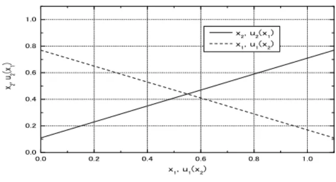
(3) 3. xi . In the game, the nodes control their packet generating rates xi and forwarding preferences pi sd to optimize their utilities; the network controls cost coefficient αi and compensation coefficient λi to maximize its revenue.. 1.0. x , u (x ) 2. 1. 1. 1. 2. 0.6. 2. 2. 1. x , u (x ). 2. x , u (x ). 0.8. 0.4. B. Nash Equilibrium 0.2. Definition 1 The situation x∗ = (x∗1 , . . . , x∗i , . . . , x∗n ) 1 is called the Nash Equilibrium in the Game Γ, if for all nodes give strategies xi ∈ Xi and i = 1, . . . , n there is Ui (x∗ ) > Ui (x∗ k xi ). (5). Remark It follows from the definition of the Nash equilibrium situation that none of the nodes i is interested to deviate from the strategy x∗i , (when such a node uses strategy xi instead of x∗i , its payoff may decrease provided the other nodes follow the strategies generating an equilibrium x∗ ). Thus, if the nodes agree on the strategies appearing in the equilibrium then any individual non-observance of this agreement is disadvantageous to such a node. In this paper, we will simplify Nash Equilibrium as NE. C. 3-Node Case Study As a simplified example, let us firstly consider an ad hoc network with 3 nodes, denoted by N1 , N2 , N3 . Transmission could be finished through one intermediate node or to the destination directly. N1 has one unit packet to send to N3 , it sends its packet to other nodes and keeps its desired cost. N2 also has packet to send to N3 . N3 has no knowledge of whether N1 or N2 will send the packet directly to it or using a relay node. (Suppose the network cannot verify any claims the nodes might make about their strategies.) Figure 1 illustrates how the Nash Equilibrium is determined by using the cost and compensation function. In this example, the packet forward probability for N 1 and N 2 are both [0,1] and both x1 versus U2 and x2 versus U1 are plotted in the same figure. The intersection point of the two plots is a Nash Equilibrium, which means both N1 and N2 can benefit each other only when they use the forward probability strategy approaching 0.5. 1. Note (x1 , . . . , xi−1 , xi , xi+1 , . . . , xn ) is an arbitrary nodes’ strategy set in cooperative game, and xi is a strategy of node i. We construct a nodes’ strategy set that is different from x only in that 0 the strategy xi of node i has been replaced by a strategy xi . As 0 a result we have a nodes’ situation (x1 , . . . , xi−1 , xi , xi+1 , . . . , xn ) 0 0 denoted by (xkxi ). Evidently, if node i’s strategy xi and xi coincide, 0 then (xkxi ) = x.. 0.0 0.0. 0.2. 0.4. 0.6. 0.8. 1.0. x , u (x ) 1. Fig. 1.. 1. 2. Nash Equilibrium in 3-Node game. III. T HE D ISTRIBUTED A LGORITHM In this section, we give an algorithm to compute NE of non-cooperative node game Γ, and illustrate the implementation issue on ad hoc networks. As mentioned above, the algorithm could easily be implemented as a local procedure (optimization of Ui (·)), once we know the node i associated cost factor αi . This is, however, based on a simple iteration method. The goal of iteration method is to search for the optimal value of of xi for problem Q. To reach this equilibrium, each node can change its strategy at a rate proportional to the iteration of its utility function with respect to its strategy, subject to constrains [16]. Moreover, since the solution to the problem Q is unique, the corresponding solutions converge to the NE vector. Here, we apply similar noncooperative distributed algorithm considered in [15] with the difference that we treat the node as link and the packet generating rate as the allocate rate. And cost and compensation parameters could be delivered to in the packet headers. For the case of more general networks, we need to calculate the derivative of the utility function of Equation 1. Then the problem is reduced to a single variable optimization problem: a node does a iterative step to compute its optimal packet generating rate. Thus, we compute the derivative with respect to equation 1, X Y dxi = x˙i = αi − P j sd dt i∈R(i). (6). j∈S(i). Note that in the above expression we first assume that the packet forwarding probabilities (p) and cost and compensation factor of all the source nodes in the network are same initially and then compute the derivative with respect to this (x). This is because during the computation the node must take both cost and compensation into account to get the optimal strategies.. −39−.

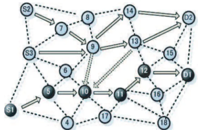
(4) 4. Thus, solving the problem is reduced to a single variable optimization issue. A node does a iterative ascent to compute its optimal packet generating rate. Thus, in its k th computation, a node i uses the iteration (k+1). xi. (k). = xi. 0. 0. + ξ(k)(C 1 (·) − KC 2 (·)). (7). where ξ(k) is a sequence of positive numbers satisfying the usual conditions imposed on the learning parameters in stochastic approximation algorithms, i.e., Σk a(k) = ∞ and Σk a(k)2 < ∞. Here, the reason we choose stochastic algorithm is that this distributed algorithm can be randomly changing with time owing to the node mobility. Thus a node needs to appropriately modify the cost function C 1 (·) and compensation function C 2 (·) based on its most recent feedback from the network. However, in case of any change in the network, there will typically be some delay till a node completely recognizes the change. Note that it is possible that different nodes settle to different local maxima. We define here that the imposed “cost and compensation” policy ensures that all the node settle Nash Equilibrium (Nash Equilibria)in the highest payoff. Above algorithm implementation requires a node to know the neighborhood status of the network around itself. In order to get effective knowledge about that in topology-blind ad hoc networks, here, we need some mechanisms (for example, we could use some discovery mechanisms) to get feedback signals and using feedback signals to measure or estimate the network status. Simply to say, the feedback signals include the node willingness to pay αi and network compensation factor λi . IV. P ERFORMANCE A NALYSIS. Fig. 2.. function (equation 1). Relay nodes observe the updating cost associated with the former packet generating rate for the new destination node. The new packet forward probability is chosen randomly. Comparing the costs and compensation the nodes choose in the next step whether to generating own packet or to forward packet for other nodes. For each node, we determined NE that results in the highest payoff function. The simulations we investigate has the main design parameters listed in table 1. We illustrate our results for various parameters. For each parameter, the default value and their varying range are provided. In our simulation, the studied scenario is high density and the speed mobility of the nodes is rather low, so we could ignore the packets drop rate. Also, we consider only the number of packets that are generated and forwarded, ignore the size of the packets, this assumption allow us to capture the main aspect of the problem and we believe it could be extended in the future work. Table 1 Main Simulation Parameters. In this section, we evaluate the performance of “cost and compensation” scheme in a general setting, which is closer to the realistic topology scenario of wireless ad hoc networks, we conducted the following simulation on NS2, using IEEE802.b at the MAC Layer.. Parameters Space Number of Nodes Placement Cost Factor Compensation Factor xi Packet size Buffer size for i Maximum xi Pjsd Simulation Time. A. Scenario and Simulation Setup We studied a given network model (Fig.2) including 20 nodes located randomly according to a uniform distribution within a geographical area of 1000m by 1000m, some nodes randomly choose a destination(e.g. S1 to D1, S2 to D2, S3 to D3), and separately generate packets according to a Poisson process with the initial value 600packet/s. At each updating step, relay nodes (e.g. 4,5,6...) decide whether to forward the packets as before, or to cease forwarding for a while. The decision is taken on the base of their current payoff. The packet forwarding graph of the random scenario. Value 1000m × 1000m 20 uniform 0∼1 0, 0.5, 1 Initial Value= 600 pacekt/s 1024byte 50 packets 2000 packet/s Initial Value=0.5 2000s. B. Metrics. −40−. We are interested in the following metrics..

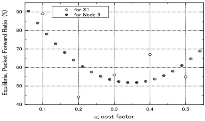
(5) 5. Equilibria, Packet Forward Ratio (%). - Equilibria on Throughput of Individual Node: Individual throughput is determined by logging the accumulative traffic originating form the node in 1s intervals. - Equilibria on Packet Success Forward Rate: computes the rate that assigned packets are successfully forwarded by node i to correct relay node or destination in 5s intervals - Convergence of the individual node strategy: computes the time required for convergence of the scheme. The individual payoff function against the time for different step size. V. R ESULTS A NALYSIS. for Node 9. 80. 70. 60. 50. 40 0.1. 0.2. 0.3. 0.4. 0.5. cost factor. Fig. 3.. Nash Equilibria for S1 and node 9. 2. Equilibria, Packet Generating Rate (10 bit/s). 70. 60. 50. 40. 30. 20. 10. 0 0.1. 0.2. 0.3. 0.4. Cost Factor (. Fig. 4.. 0.5. ). Convergence of S1 behavior. 1.0. 0.9. 0.8. Global Convergence. In evaluation, S1 is selected, as it is the most extreme source node in the network; and node 9 is also selected as it could represent the mobile nodes near the center of the network, which are frequently used as relay nodes. In Fig.3, the equilibria strategy is calculated for node S1 and 9, cost factor α is ranging from 0 to 0.6, compensation factor is set to 1. It is shown that the value of Equilibria on packet success forward ratio for node S1 and 9 can be selected to find the best tradeoff between individual payoff and packet forwarding probability for other similar location nodes. As α = 0.1, for node 9, the equilibria points are smaller. This is due to the fact while node 9 is closet to the center of the network, distances to its neighboring nodes are all relatively high, and will be carrying larger amounts of traffic for other nodes. Hence, when α = 0.5 its usage and equilibria points will be reasonably high, as reflected by the figure. As the Fig.4 indicates S1 has a steady state under different cost and compensation value. Even if convergence rate is only weakly fluctuated by compensation function, we still could see the node behavior can be influenced through the introduction of a compensation function. It can be observed from Fig.5 that the final behavior of node 9 converges under the control of proposed system, here different α, λ values are used. As we could see that small values of α lead to low iteration steps. This is due to the fact that if the traffic is low, nodes will operate far from the central region and their strategies will not be strongly coupled. However, as the value of α increases, the convergence speed also increases, even not so obvious. This is due to the fact that as α increases, the cost is heavier, more negotiation time is needed to compensate for the packet forward probability strategies. Accordingly, there is less incentive for the nodes behave selfishly. This figure also compares payoff as a function of the cost factor α with different λ value. We see that through the compensation function the NE strategies, convergence time for node 9 is much longer than. for S1. 90. 0.7. 0.6. 0.5. 0.4. 0.3. 0.2. 0.1. 0.0 0. 200. 400. 600. 800. 1000. 1200. Simulation Time (s). Fig. 5.. −41−. Convergence of node 9 behavior. 1400. 1600. 1800. 2000.

(6) 6. only using cost strategies, thus choosing cooperation is more beneficial with respect to non-cooperative behavior. Also, payoff function for node 9 increases with the high compensation factor. VI. C ONCLUSION AND F UTURE W ORK We established a framework using game theory to provide incentives for non-cooperative nodes to collaborate in the case of wireless ad hoc networks. The incentive scheme proposed in the paper is based on a simple “cost and compensation” mechanism via pricing that can be implemented in a completely distributed system. Using non-cooperative game model, we showed network has a steady state and such optimal point — NE exist in the system, the algorithm we provided helps to find the NE. From the simulation results, we showed that node behavior could be influenced through the introduction of “cost and compensation” system. The advantage of this proposed scheme is to lead to a less aggressive way in the sense that it does not result in a degenerate scenario where a node either generates all the own traffic, not forwarding any of the request, or forwards all the other nodes packets. As far as we know, this is the first work that introduce ”cost and compensation” concept that has formal framework of encourage nodes to cooperate. In terms of future work, we will investigate the effect of different packet sizes on our scheme, and take the dynamic number of arrival and departure nodes into consideration. However, in this paper we do not discuss the conditions under which integration of nodes are interested in forming small non-cooperative groups, this will need a strong NE exist in the system, but it rarely happens. We think this problem will be a part of our future work. Our future work will also want to address the issues of the algorithmic implementation in the context of different measurement scenarios.. [5] K. Paul and D. Westhoff, “Context Aware Detection of Selfish Node in DSR based Ad-hoc Network”, IEEE GLOBECOM 2002, Taipei, Taiwan, Nov. 2002 [6] S. Buchegger, J.-Y. Le Boudec,“Performance Analysis of the CONFIDANT Protocol: Cooperation Of Nodes - Fairness In Distributed Ad-hoc NeTworks” MobiHoc 2002, Lausanne, 911 June 2002 [7] Sergio Marti, T.J.Giuli, Kevin Lai, and Mary Baker, “Mitigating Routing Misbehavior in Mobile Ad Hoc Networks”, Proc. of Mobicom 2000, Boston, August 2000 [8] Luzi Anderegg and Stephan Eidenbenz,“Ad hoc-VCG: a Truthful and Cost-Efficient Routing Protocol for Mobile Ad hoc Networks with Selfish Agents”, Mobicom San Diego,California,Sep.2003. [9] Chiranjeeb Buragohain, Divyakant Agrawal, Subhash Suri,“A Game Theoretic Framework for Incentives in P2P Systems” Proc. of the Third International Conference on P2P Computing (P2P2003), Linkoping Sweden, 2003 [10] J. Crowcroft, R. Gibbens, F. Kelly and S. Ostring, “Modelling Incentives for Collaboration in Mobile Ad Hoc Networks” Proc. of Modeling and Optimization in Mobile Ad Hoc and Wireless Networks (WiOpt)2003, March 3-5, 2003, INRIA Sophia-Antipolis, France [11] P. Michiardi and R. Molva, “ game theoretical approach to evaluate cooperation enforcement mechanisms in mobile ad hoc networks” Proc. of Modeling and Optimization in Mobile Ad Hoc and Wireless Networks (WiOpt)2003, March 3-5, 2003, INRIA Sophia-Antipolis, France [12] S.H. Shah, K. Chen, K. Nahrstedt, “Dynamic bandwidth management for single-hop ad hoc wireless networks”, Proc. IEEE International Conference on Pervasive Computing and Communications (PerCom 2003), Dallas-Fort Worth, Texas, USA, Mar. 2003. [13] J. Yoon, M. Liu, B. Nobel, “Random waypoint considered harmful”, Proc. of the 22nd Annual Joint Conference of the IEEE Computer and Communications Societies (InfoCom 2003), San Francisco, CA, USA, Mar.-Apr. 2003. [14] Haikel Yaiche, Ravi R. Mazumdar, Catherine Rosenberg,“A game theoretic framework for bandwidth allocation and pricing in broadband networks”, IEEE/ACM Transactions on Networking, 2000, Volume 8 , Issue 5 , Pages: 667 - 678. [15] Zuyuan Fang and Brahim Bensaou,“Fair Bandwidth Sharing Algorithms based on Game Theory Frameworks for Wireless Ad-hoc Networks”, Infocom 2004, [16] J.B.Rosen, “Existence and uniqueness of equilibrium points for concave n-person game,” Econometrica, vol.33,pp.520-534, Jul.1965.. R EFERENCES [1] Levente ButtyLan, Jean-Pierre Hubaux, “Stimulating Cooperation in Self-Organizing Mobile Ad Hoc@Networks” ACM/Kluwer Mobile Networks and Applications (MONET), 8(5), Oct., 2003 [2] Vikram Srinivasan, Pavan Nuggehalli, Carla F. Chiasserini, Ramesh R. Rao, “Cooperation in Wireless Ad Hoc Networks” Proc. of IEEE INFOCOM, San Francisco March 30 April 3, 2003 [3] Pietro Michiardi and Refik Molva, “Simulation-based Analysis of Security Exposures in Mobile Ad Hoc Networks”, European Wireless Conference, 2002. [4] Sheng Zhong, Jiang Chen, and Yang Richard Yang,“Sprite: A Simple, Cheat-Proof, Credit-Based System for Mobile Ad-Hoc Networks” Pro. of IEEE INFOCOM 2003, San Francisco, CA, April 2003.. −42−.

(7)