Recent advances on 1-cocycles in the space of knots (Intelligence of Low-dimensional Topology)

Recent advances

on

1-cocycles

in the space of knots

Arnaud Mortier

OCAMI, Osaka City University

Abstract

Thisisasurvey of two recent papers[8, 13]inwhichwereintroducednewmethods forconstructing 1-cocyclesin the space of knots. The construction from [13] isanatural adaptation of Polyak-Viro’s formulas for finite-type knotinvariants;it isconjecturedtogivethe firstcombinatorial formulas for$\mathbb{Z}-$ valued Vassiliev 1-cocycles. In [8], the cocycles take valuesin skein modules associated withquantum knot invariants; conjecturally, the examples produceddetect information regardingthe geometry of knots.

Fora broader panoramaon this topic, see also [6, 7, 15, 16, 19], Sections 1.6-1.8 of [5], and [9] whichis a sequel to [8],

1

Finite-type

1-cocycles

of

knots given

by

Polyak-Viro formulas

[13]

Vassiliev’s cohomologyclasses

were

introduced in 1990, at

a

time when the cohomology of

the spaceof knotshadbarely been studied. Intheyears that followed, two kinds ofexplicit

formulas were proved to describe all of Vassiliev’s $0$-cocycles, best known as finite-type

invariants: anintegral formula, due to Kontsevich [12], andpurely combinatorial formulas

due to Polyak-Viro [14] (see also [10]).

In the meantime, in higher degree, only one example was proved to exist, by Teiblum

and Turchin (at the time a student of Vassiliev), and this 1-cocycle $v_{3}^{1}$ waited unti12001

before Vassiliev [19] found how to actually evaluate it, over $\mathbb{Z}_{2}$, with a combinatorial

formula involvingdifferential geometry. Ten years later, Sakai [15] described

a

realization

of$v_{3}^{1}$ over $\mathbb{R}$ by

means

of an integral formula.

The purpose of [13] is to fill the gap of amissing combinatorial formula for $v_{3}^{1}$ over $\mathbb{Z},$

to

remove

geometric conditionsfrom the computation process, and to findmore examples

of 1-cocycles. Just like the original works of Vassiliev [17, 18], this article considers the

space of smooth long knots–i.e., embeddings $\mathbb{R}\mapsto \mathbb{R}^{3}$

that

are

standard outside of $[0$,1$].$

1.1 Preliminary: Gauss diagram formulas (after [14])

Thespirit of Polyak-Viro’s Gauss diagramformulas is to count the subdiagrams ofaknot,

with weights. Here, knot diagrams arerepresented combinatorially using Gaussdiagrams

-see

Fig.1, and a subdiagram is the result ofremoving $a$ (possibly empty) set of

arrows.

One ofthe origins of that idea lies in the well-knownformula for computing the linking

number of a 2-component oriented link: given a link diagram, $lk(L_{1}, L_{2})$ is the sum of

crossing is

a

subdiagram with only

one

arrow

remaining, oriented from $L_{1}$ to $L_{2}$, andthe

weight given to each subdigram is the writhe ofthe crossing.

In [14], Polyak and Viro give such formulas for computing (among others) the first two

Vassiliev invariants (Theorems 1 and 2). In both

cases

(as well

as

in the linking number

formula), the weight given to asubdiagram is equal to the product of its writhe numbers,

times a constant which depends only

on

theunderlying unsigned diagram. Suchparticular

choices of weights proved to be extremely

common

in further literature (see for instance

[3, 2, 4 and yield what is often called

arrow

diagram

_formulas

(an

arrow

diagram is

a

Gauss diagram deprived from its decorating signs).

$\nearrow^{\cross+\backslash }$ $/_{-}\backslash ^{\nearrow}$

$\sim$

$\cross^{\backslash }$

Figure 1: Along figure eight knot diagram and its Gauss diagram

Figure 2: Example of computationof the Casson invarianton arandomGauss diagram

The main interest of these formulas lies in the following result.

Theorem 1 (Polyak-Viro [14], Goussarov [10]). A knot invariant admits

a

Gauss diagram

formula

if

and only

_if

it is

a

Vassiliev invariant.

Although the proof given by the authors of this theorem does not mention the original

definition of Vassiliev invariants, it is possible to obtain such formulas by computing

weight systems (see [1]) and integrating them via the homological calculus presented in

[19]. This process highlights the deep origin ofthe writhe numbers in these formulas,

as

co-orientations of singular strata in the space of all (including singular) knots. It is also

one reason to believe that computing products of writhes at a higher level could yield

formulas for Vassiliev 1-cocycles.

1.2 Arrow germ formulas

The idea in [13] is to copy Polyak-Viro’s construction using

as

raw

material not a Gauss

diagram, but

a

Reidemeister move, which is here regarded

as an

elementary path in the

Definition 1. An $i$-germ $(i=1,2,3)$ is

a couple

_of

Gauss diagrams that

_differ

only by a

Reidemeister$i$

move.

$A$ partia13-germ is a 3-ge7m with

one

arrow

removed (in both diagrams)

_from

the

Reidemeister triple.

$A$ subgerm is the result

of

removing a set

_of

arrows

_from

$a$ (possibly partial)

germ,

con-sistently in both diagrams.

Arrows

involved in the Reidemeister

move

cannot be removed,

except in 3-germs where at most one

arrow

_from

the triple can be forgotten.

As before, these notions have a counterpart with no sign decorations, called (partial)

arrow

$germs-and$ as before, the latter

are

meant to count subgerms, weighted with the

product of writhes of the

arrows

involved.

The main result of [13] is the following.

Theorem 2. The

_formal

sum

$\alpha_{3}^{1}$

of

(partial)

arrow

germs

on

Fig.3

_defines

$a$ 1-cocycle

in the space

_of

long knots,

over

$\mathbb{Z}$

. Its reduction mod 2 coincides with Teiblum-Turchin’s

cocycle $v_{3}^{1}.$

The second statement is proved by showing directly that $\alpha_{3}^{1}$ mod2 is “of finite type”,

using Vassiliev’s homological calculus presented in [19]. The proof of the first

state-ment relies on a higher order Reidemeister theorem, that is,

an

exhaustive list of all

2-codimensional strata corresponding to the most generic degeneracies of Reidemeister

moves

(by definition, a 1-cocycle should vanish on the meridians of such strata). A

com-plete description of those strata and their meridians is given in [13]; see also [7].

Notation:

Figure3: The first non-trivialarrowgerm formula$\alpha_{3}^{1}$: three partialarrow3-germsandonearrow 3-germ

As one

can

see, no 1- or 2-germs

are

involved in the formula of Theorem 2, and this

is actually

a

general fact: in any cohomology class represented by germ formulas, there

is a formula which contains only (possibly partial) 3-germs ([13], Proposition 2.8). As a

result, the linear system with germs as variables and 2-meridians as equations is reduced

to a reasonable size ([13], Theorem 2.11).

Conjecture 1. Every 1-cohomology class with an arrow germ presentation is

_of

_finite

type in the sense

_of

Vassiliev.

So far, only

one

way is known for proving that a 1-cocycle is of finite-type over $\mathbb{Z}$;

it consists in defining orientations on the varieties involved in Vassiliev’s homological

1.3 Evaluation of$\alpha_{3}^{1}$

on

canonical cycles

One interest of 1-cocycles is that evaluating them

on

loops that

are

defined canonically

for all knots produces knot invariants. The easiest example ofsuch aloop, for long knots,

is the loop rot (K) which consists of a full positive rotation of $K$ around its axis–see

Figs.4 and 5. It is proved in [13] that $\alpha_{3}^{1}(rot(K))$ is equal to minus the Casson invariant

of $K$:

$\alpha_{3}^{1}(rot(K))=-v_{2}(K)$.

This equality

was

conjectured to hold for the Teiblum-Turchin cocycle in [16]. Turchin’s

conjecture would follow from the above result and Conjecture 1.

Figure4: One realization of the looprot(K) as asequence of Reidemeister moves

Figure5: Therailwayfollowed by $K$onFig.4 is isotopictoafull rotationaround the axis

A result of Hatcher [11] states that besides rot(K), there is essentially only

one

other

interesting loop in the moduli space of all long knots equivalent to

a

given prime knot.

This second loop, often called the Hatcher loop Hat (K), consists of sliding alittle “ball at

infinity”’ along a fixed parametrization ofthe knot in$\mathbb{S}^{3}$

(a framing convention should be

made, because every time the ball makes a full spin arounditself, it adds $\pm rot(K)$ to the

loop). Although it does not

seem

easy to evaluate $\alpha_{3}^{1}$ on Hat (K), further investigation

showed that there is another

arrow

germ

formula $\tilde{\alpha}_{3}^{1}$, with the

same

properties

as

$\alpha_{3}^{1}$

so

far, and such that if $K$ has framing $0$, then

$\tilde{\alpha}_{3}^{1}$(Hat (K) )

$=-6v_{3}(K)$

.

Here$v_{3}$ denotes the only Vassiliev invariant of order 3 with value 1 on the positive trefoil,

$-1$ on _{the negative trefoil and} $0$ on the unknot. This result is to appear in asubsequent

2

Quantum

one-cocycles

for knots [8]

In this article, Fiedler defines a

new

family of 1-cocycles in the topological moduli space

oflong knots, which are then extended to cocycles in the space of string links. As in the

previous article (Section 1), the formulas are constructed as algebraic intersection forms

with the variety of Reidemeister moves, purely combinatorially: follow aloop in the space

of knot diagrams, and every time you meet a Reidemeister move, count something. Only

thistime what you countdoes not livein

a

“small” group like$\mathbb{Z}$

, but in

a

more

complicated

structure that stays closer to topology and keeps

more

information.

One of the motivations here is to detect geometry-related information, with the

fol-lowing result in mind (see the definitions of rot and Hat in the previous section).

Theorem 3 (Hatcher [11]). Let $K$ be a long knot which is not a satellite. Then the loops

rot (K) and Hat (K)

are

linearly independent over $\mathbb{Q}$

if

and only

_if

$K$ is hyperbolic.

It

means

that if one can create a 1-cocycle powerful enough to detect exactly when

rot (K) and Hat (K)

are

linearly dependent, then it gives

a

simple criterionto evaluate the

geometry of prime knots. The ultimate goal in that direction is to find

a

cocycle $v$ such

that the quotient v(rot)/v(Hat), when not arational number, is related to the hyperbolic

volume.

2.1 The space of cochains

There

are

alot of combinatorial tools required to define properly the objects in Fiedler’s

theory; we begin with a simplified version, which will be refined gradually in the next

subsections. In particular, we first set aside orientation and sign issues.

Let us describe the elementary cochains from which one tries to obtain 1-cocycles.

They

are

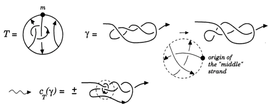
based on a simple surgery operation that generalizes knot mutations. Indeed,

let $T$ be a tanglediagram in a2-disc, with 6 boundary points. One defines anelementary

cochain $c_{T}$ as follows. Pick a generic path $\gamma$ in the space of long knot diagrams. For

each Reidemeister III move involved in $\gamma$, notice that the local Reidemeister picture is a

tangle diagram in a disc, with 6 boundary points; remove that disc from your diagram,

and replace it with $T$, making sure that the boundary points match; there are six ways

to do that, and we will explain later how to choose

one

canonically. The evaluation $c_{T}(\gamma)$

is by definition the formal

sum

of all tangle diagrams

so

obtained.

By considering tangles with 4 (respectively, 2) boundary points,

one can

similarly

construct cochains that detect Reidemeister II (respectively, I)

moves.

Now ifone stops here, thespaceof cochains is indexed by tangles in a disc, so that it is

infinite-dimensional.

Moreover, abrief examination reveals that therearevery few chances

to ever find a cocycle in that space: indeed, a 1-cocycle should vanish

on

2-meridians,

and it is not easy for a formal sum of tangle diagrams to vanish (even with proper signs

defined). The natural

answer

to both these issues is to push the values of the cochains

in a skein module. In [8], two modules are separately considered: the HOMFLYPT and

Kauffman polynomials, which both yield finitely generated cochain spaces. Note that in

へ_{$\sim$ $c_{T}(\gamma)=$}

Figure6: Elementarycochainassociated with an oriented tangle$T$. The middlestrand issueis explained

in Subsection 2.1.3.

2.1.1 Local and globaltypes

An empiricalfact in this theoryis that 1-cocycle formulas tend to contain

a

lot of

symme-try, and themoresymmetry there is inaformula, themorelikely it isto be cohomologically

trivial. There are mainly two ideas in [8] to get round this difficulty: first,

use

parameters

and decorations

so as

to break the symmetry

as

much as possible; second, find

a

way to

extract interesting information

even

from

a

cocycle that is cohomologically trivial (see

Section

2.2.1).

Let us

assume

for now that

we

work with long knot diagrams (see example

on

Fig.1).

There are a number of data that

one

can

read given a Reidemeister

move

in such

a

diagram, which together define the local and global types of the move. Then, if$l$ denotes

one particular local type, and $g$ a global type,

one

can enrich the previous settings by

defining an elementary cochain $c_{T,l,g}$: it makes the

same

computation as $c_{T}$ but only if

the Reidemeister

move

has type $(l, g)$ (so that $c_{T}$ is the

sum

of $c_{T,l,g}$

over

all types

$l$

and $g)$

.

Local types

are more

conveniently read

on

the local knot diagram picture, while global

types require to look at how the involved crossings

are

arranged

on

the Gauss diagram,

with respect to each other and to the point at infinity; the point at infinity appears to be

the key to break the symmetry and allow non-trivial solutions to exist.

Figure

7 sums

up the definitions of all types, and where to find them in [8].

Terminology. Thenotation $c_{T,l,g}$

”

, althoughconvenient for

an

overviewof the article,

is not the one used in [8]. There, cochains

are

systematically defined by giving, for each

coupleoftypes $(l, g)$_, which tangles$T$ (calledpartialsmoothings) contribute. Forinstance,

“for the cochain $R$, the partial smoothing $T_{r_{c}}$ for type 3 is

means

in the current

terminology that $R$can be written

$R=c$

Figure 7: All local and global typeswiththeirreference pagesin [8] (version 2)

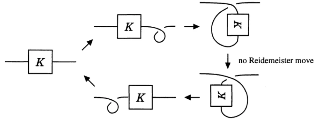
2.1.2 Signs

One obvious necessary condition for a cochain $c$ to define a 1-cocycle is that $c$ should

vanish

on

any little loop in which

one

Reidemeister

move

is performed and then undone.

As a result,

one

must either work

over

$\mathbb{Z}/2$,

or

define “co-orientations” of Reidemeister

moves.

The latter choice is made in [8],

as

follows.

In the

case

of Reidemeister I and II moves, the evaluation of an elementary cochain

$c_{T,l,g}$

comes

with

an

additional minus sign if and only if the

move

destroys crossings.

In the case of Reidemeister III, the co-orientation is defined separately for each local

type. That is the meaning of $the+and-$ signs in [8] Fig.16 p.31, they indicateon which

side of the

move

each picture is. When evaluating a cochain, count an additional minus

sign if and only if the

move

goes from the positive to the negative side. Note that the

signs here were not chosen arbitrarily. The easiest way to show it might be to point out

that in Fig.8, where every local type appears exactly once, all eight triangles

are on

their

1

Figure8: All eight local types ontheir positiveside, inonepicture

2.1.3 Gluing conventions

We

now

explain how Fiedler chooses

one

out of six ways of gluing

a

graft tangle after

removing a Reidemeister III tangle (for $R$I there is nochoice since the skein modules are

1-dimensional, and for R II it is directly made clear on each picture, like [8] Fig.41 p.59,

which in

our

current notations would read $-(v-v^{-1})c$)$(,+,0)$

.

First, notice that for local types 2 and

6

(called star-like),

sources

and sinks alternate

along the boundary of the Reidemeister tangle; for the remaining (braid-like) types 1,

3, 4, 5, 7 and 8, the

sources

can be grouped together

on

one side of the disk. In the

latter case, the convention is that the three boundary points at the

_left

ofany picture of

agraft tangle $T$ should replace the three

sources

of the removed tangle. This convention

is especially useful when working

over an

unoriented skein module; otherwise, the simple

fact that orientations should match leaves no choice.

For local types 2 and 6, one defines the mid point in the Reidemeister tangle as

the

source

of the “middle strand, which goes neither

over

the two other strands,

nor

under them. The convention is then to decorate one of the boundary points in the graft

tangles with a letter $m$”, indicating that this point always replaces the mid point when

performing

a

surgery–see Fig.6.

When working

over an

oriented skein module, only graft tangles with consistent

orien-tations

are

allowed; note that this consistency condition depends

on

the local type.

2.1.4 Weights

There are two major ingredients in Fiedler’s formulas. The first is the idea ofperforming

surgeries that formally depend on

some

local and global parameters, i.e., the cochains

$c_{T,l,g}$ defined so far. The second is to weight these cochains with Gauss diagram

formulas. Very roughly, it amounts to considering the module freely generated by the

elementary cochains $c_{T,l,g}$, not over

$\mathbb{Z}$, but over a ring of arrow diagrams (as defined in

Section 1).

Asin Section1, those

arrow

diagramscompute

sums

of productsofwrithes in theGauss

diagram that represents the long knot at the moment where each Reidemeister

move

is

performed. The number of writhes involved in each product determines the degree ofthe

2.2 Results

Recall that when a 1-cochain in the space of knots isdefined as an intersectionform with

Reidemeister moves, the condition for being a cocycle is to vanishon the meridians of the

2-codimensional strata defined by the higher order Reidemeister theorem (just like knot

invariants, i.e., $0$-cocycles, should vanish

on

the meridians of the 1-codimensional strata

defined by the usual Reidemeister theorem). Two of these strata are by far the most

complicated, and occupy acentral place in [8]:

$\bullet$ The set of

knots whose projection to the plane contains a quadruple point (which

can

be thought of as an

arc

sliding over a Reidemeister III move), denoted $by*.$

The equations associated with their meridians are called the tetrahedron equations.

$\bullet$ The set

ofknots whose projection contains

a

triple point withtwo tangent branches

(an arc sliding over/under/through a Reidemeister II move), denoted by $\succ|\prec$

.

The

associated equations

are

called the cube equations.

The results

are

organized as follows: for each skein module (HOMFLYPT, pp.34-149

and Kauffman, pp.149-168), two 1-cocycle

formulas

are

constructed: $R_{\eta eg}^{(1)}$

and $\overline{R}^{(1)}$ in the

HOMFLYPT

case, $R_{F,reg}^{(1)}$ and $R_{F}^{-(1)}$

in the Kauffman

case.

Each of these

are

built

step by step, by first _{solving the tetrahedron equation, then adjusting the solution so}

that it satisfies also the cube equations, then adjusting again so as to get all (when

possible) remaining equations satisfied. Formulas whose

name

contains a subscript “reg”

do not vanish

on

meridians involving Reidemeister I moves; however they vanish on all

other meridians, which makes them regular cocycles, i,e., invariants of regular loops up

to regular isotopy ([8] Theorem 3 p.94); they are both made of quantum cochains with

linearweights. Onthe other hand, $R^{(1)}-$

and$R_{F}^{-(1)}$

satisfy all equations and define non-trivial

cocycles in the space of long knots ([8] Theorem 4p.127 and Theorem 5 p.165). They are

made of amain part which is a quantum cochain with (at most) quadratic weights, and

a _{corrective term which purely consists ofa weight ofdegree 3 (and no surgery part).}

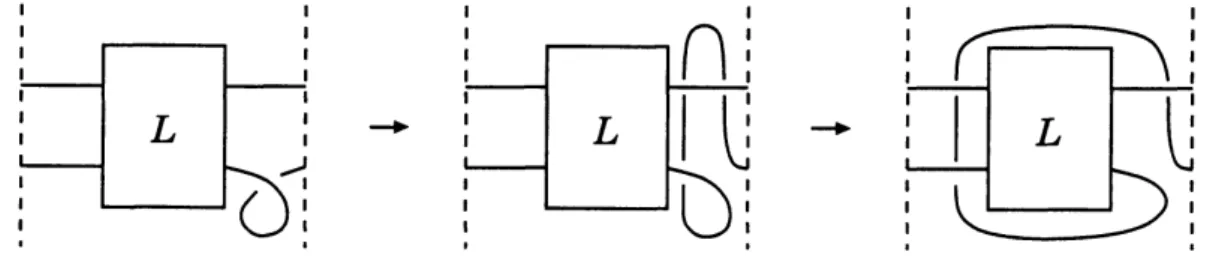
2.2.1 From long knots to string links

There

are

many

reasons

for which

one

would like to generalize a construction related to

long knots to string links in a 3-ball. For instance, producing families of invariants via

knot cabling, or generalizing a formula computing the trivial knot invariant, which may

prove to be non-trivial when applied to string links. When it comes to 1-cocycles, tangles

ingeneral are a little bit unfriendly: the moduli space of all tangles isotopic to agiven one

has very often a trivial first homology group. However, even a 1-cocycle formula that is

null-cohomologous can lead to non-trivialinvariants of tangles if evaluated on a canonical

arc which is not a loop.

The way Fiedler extends his long knot cocycle formulas to arbitrary string links is

extremely simple: just like knots, string links can be represented with Gauss diagrams,

the only difference is that the base manifold is not a circle, but a collection of numbered

arcs.

Fix arbitrarily:

2.

a

point at infinity

among

the gluing points.

That is all. Now any sequenceofReidemeister

moves

applied toanystringlink diagram

looks like a sequence applied to a long knot, and it makes

sense

to evaluate Fiedler’s

formulas there. Any quantum cocycle for long knots defines a family of cocycles in the

moduli space _{of string links, indexed by} the above choices of

a

circular permutation and

apoint at infinity.

2.2.2 The scan-arc and the scan-property

As mentioned earlier, there

are no

non-trivial loops in the moduli space ofstring links in

general, except for particular

cases

such

as

longknots and their cables (for which there is

a version of the Hatcher $1oop-[8]$, p.8).

Fiedler introduces a scan-arc, defined canonically for all string links, and denoted by

scan

(L). We represent it

on

Fig.9. It

can

be thought of

as a

generalization of the loop

rot (K) defined for long knots: indeed, rot (K) consistsbasically of twoconsecutive $\langle$

scans”

(Fig.4). Notice that the little loop on the first frame is not a part of the string link, and

its “creation” by Reidemeister I is not apart of the

scan-arc

either (although the sequence

of Reidemeister II

moves

that lead to the second frame is included in the scan-arc): it

follows that the

scan-arc

is regular (it does not involve any Reidemeister I move), hence

it makes

sense

to evaluate $R_{veg}^{(1)}$

and $R_{F,reg}^{(1)}$ there.

$arrow$ $arrow$

Figure 9: Thescan-arcofastringlink $L$

Now

one

would like

a

result of the type “Let $c$ be

a

quantum cocycle formula. Then

$c(scan(L))$ is

an

isotopy invariant of the string link L.” It is not difficult to

see

that this

holds true if$c$is aquantumformula with constant weights. However itfailswith arbitrary

weights.

By definition, aquantum cocycle formula$c$issaid to have the scan-property if$c(scan(L))$

defines an isotopy invariant of the string link $L$

.

All four formulas constructed in [8] have

that property ([8] Theorems 3, 4, 5).

Among many examples, let usmentionthat if$L$is chosen to bethepositive generatorof

the 2-strand braidgroup,andif the point at infinity is chosen correctly, then $R_{7eg}^{(1)}(scan(L))$

is equal to the HOMFLYPT polynomial of the right trefoil (times the class of the trivial

braid in the HOMFLYPT skein module).

As for $\overline{R}^{(1)}$

, the computations made lead to the following conjectures ([8], Conjectures

1 and 2).

its

HOMFLYPT

polynomial. Let $\delta$

denote the

HOMFLYPT

polynomial

_of

the trivial

2-component link. Then

$\overline{R}^{(1)}$

(rot (K) ) $=\delta v_{2}(K)P_{K}.$

Conjecture 3. Let $K$ be

a

long

_knot

_{with trivial}

_framing

and with

non

trivial

Casson

invariant. Then $R^{(1)}(Hat(K))$ _{is a}

_non

_zero

_{integer multiple}

of

$R^{(1)}(rot(K))-$

if

and only

if

$K$ is a torus _knot.

So far those two conjectures have been checked for knots up to 4 crossings.

2.2.3 Gradings

One specificity ofthe

formulas

$R_{eg}^{(1)}$

and $R_{F,reg}^{(1)}$ extended to string links

is that they

can

be refined into a collection of cocycle formulas $R_{\tau eg}^{(1)}(A)$ and

$Rreg$) (A) indexed by a set of

gradings, sothat the original_formulas

_are

_the

_sum

_{of the refined formulas}

_over

_{all possible}

gradings.

A grading is defined for any

Reidemeister

II or III

move.

Just like $c_{T,l,g}$ is oblivious of

Reidemeister

moves

that

are

not of type $(l, g)$, $R_{\gamma eg}^{(1)}(A)$ and$R_{Fre}^{(1)}(A)$ disregard the

moves

that do not have grading $A$

.

The full

definition, however, is not very enlightening, so

we

do not mention it here;

see

[8], Definition 9 p.48.

References

[1] Dror

Bar-Natan.

_{On the Vassiliev knot invariants. Topology, $34(2):423-472$,}

_1995.

[2] Michael Brandenbursky. Link invariants via counting surfaces. ArXive-prints,

September

2012.

[3] _{Sergei Chmutov, Michael Cap Khoury, and Alfred Rossi. Polyak-Viro formulas for}

coefficients of the Conwaypolynomial. J. Knot TheoryRamifications, $18(6):773-783,$

2009.

[4] Sergei

Chmutov

and Michael Polyak. Elementary combinatorics of the

HOMFLYPT

polynomial. Int. Math. Res. Not. IMRN, (3):480-495,

2010.

[5] _{Thomas Fiedler. Gauss} diagram invariants

_for

knots and links, volume 532 of

Math-ematics and its Applications. _{Kluwer Academic Publishers, Dordrecht, 2001.}

[6] Thomas Fiedler. Isotopy invariants _{for closed braids and almost closed braids via}

loops in

stratified

spaces.

_{ArXiv Mathematics}

$e$-prints, June

2006.

[7] Thomas Fiedler. Knot polynomials via one parameter knot theory. ArXiv

Mathe-matics $e$-prints, December 2006.

[8] Thomas Fiedler. Quantum one-cocycles forknots (v2). ArXiv Mathematics $e$-prints,

Apri12013.

[9]

Thomas

_{Fiedler. Singularization of knots and closed braids.}

_ArXiv

$e$-prints, May

[10] Mikhail

Goussarov.

Finite-type invariants

are

presented by

Gauss

diagram formulas,

1998. Ranslated from Russian by Oleg Viro.

[11] Allen Hatcher. Spaces of Knots. ArXiv Mathematics $e$-prints, September 1999.

[12] MaximKontsevich.

Vassiliev’s

knot invariants. In I. M.

_Gel’fand

Seminar, volume

16

of Adv.

Soviet

Math., pages

137-150.

Amer. Math. Soc., Providence,

1993.

[13] Arnaud Mortier. Finite-type 1-cocycles ofknots and virtual knots given by

Polyak-Viro formulas. Available at https:$//$sites.google.com/site/mortier2xO/home/

publications thesis and-preprints.

[14] Michael Polyak and Oleg Viro. Gauss diagram formulas for Vassiliev invariants.

Internat. Math. Res. Notices, (11):445ff., approx. 8 pp. (electronic),

1994.

[15] Keiichi Sakai. An integral expression of the first nontrivial one-cocycle of the space

of long knots in $\mathbb{R}^{3}$

.

_Pacific

J. Math., $250(2):407-419$, 2011.

[16] Victor Turchin. Computation of the first nontrivial 1-cocycle in the space of long

knots. Mat. Zametki, $80(1):105-114$,

2006.

[17] Victor A. Vassiliev. Cohomology of knot spaces. In Theory

_of

singularities and

its applications, volume 1 of Adv. Soviet Math., pages 23-69. Amer. Math. Soc.,

Providence, RI, 1990.

[18] Victor A. Vassiliev. Complements

_of

discriminants

_of

smooth maps: topology and

ap-plications, volume

98

of Translations

_of

Mathematical Monographs. American

Math-ematical Society, Providence, RI, 1992. Translated from theRussian by B. Goldfarb.

[19] Victor A. Vassiliev. Combinatorial formulas for cohomology of spaces of knots. In

Advances in topological quantum

_field

theory, volume 179 ofNATO Sci. Ser. II Math.

Phys. Chem., pages 1-21. Kluwer Acad. Publ., Dordrecht, 2004.

OCAMI, Osaka City University

3-3-138

Sugimoto, Sumiyoshi-ku, Osaka-shi

Osaka 558-8585,

JAPAN