Hyperfunctions and Cech-Dolbeault cohomology in the microlocal point of view (Microlocal analysis and asymptotic analysis)

全文

(1)7. Hyperfunctions and Čech‐Dolbeault cohomology in the microlocal point of view By. Naofumi HONDA. *. Abstract. In this note, we explain how to construct the boundary value map. Sato hyperfunction in the framcwork of Čech‐Dolbeault cohomology.. b_{\Omega}. : \mathscr{O}(\Omega)arrow \mathscr{B}(M) of. s. §1.. Introduction. The boudnary value map b_{\Omega} is the most important morphism in the hyperfunction theory, by which we can understand a hyperfunction to be the sum of boundary values of holomorphic functions defined on wedges along a real analytic manifold. As was. explained in [2] of this volume, the theory of Čech‐Dolbeault cohomology brings several benefits to the treatment of a hyperfunction, and as such an important example, we here explain how to construct the boundary value morphism in our framework. For an. application to the theory of Laplace hyperfunctions, see [3] in this volume. This is a joint work with Takashi Izawa and Tatsuo Suwa. §2. Let. M. Boundary value morphism. be a real analytic manifold assumed to be orientable and countable at infin‐. ity, and let. X. be its complexification. Note that, through the note, we use the same. notations as those in [2] of this volume. Let. \Omega. be an open subset in. X,. for which we introduce the following two conditions:. \overline{\Omega}\supset M.. (B1). (B2) The inclusion (X\backslash \Omega)\backslash M\mapsto X\backslash \Omega gives a homotopy equivalence. 2010 Mathematics Subject Classification(s): Primary *. 32A45 ,. Secondary. Supported by JSPS Grant 18K03316 Faculty of Science, Hokkaido University. Sapporo 060‐0810. Japan. [email protected] jp.. 32C35..

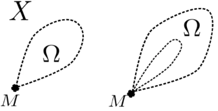
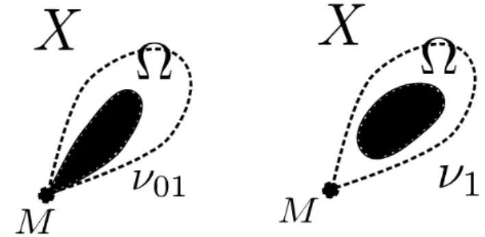
(2) 8. NAOFUMI HONDA. For example, a usual convex wedge. \Omega. along. M. like a left shape in Fig. 1 satisfies the. condition (B_{2}) . However, the right shape in the same figure that is a wedge along in which the smaller one is removed violates. connected components while. N. X\backslash \Omega. (B_{2}). because. (X\backslash \Omega)\backslash M. M. consists of two. is connected.. ’. \prime^{\prime^{\prime^{\prime^{t} \backslash} .-\sim_{s_{\backslash} .. l^{\prime^{\prime^{\prime'} ,. 1. e^{\prime^{e\backslash}.\ovalbox{\t\smal REJ CT}.-\ovalbox{\t\smal REJ CT}\backslash.. \Omega \prime 1. M\buletprim.\ elprim'\ eprim'\ elprim\ e. Omga\prie m\prie, m'\prie^{ m'}\prie ’. Figure 1. A good case (left) and bad case (right).. Set. \mathcal{W}=\{V_{0}=X\backslash M_{:}V_{1}=X\}. and. In what follows, we always assume that. \mathcal{W}'=\{V_{0}\} . \Omega. We also set V_{01}=V_{0}\cap V_{1} as usual.. satsifies the above two conditions. Then we. will define the following boundary value map b_{\Omega}. :. \mathscr{O}(\Omega)arrow \mathscr{B}(M)=H_{M}^{n}(X;\mathscr{O})\otimes_{Z_{M} (Af)}or_{II/X}(M). \simeq H_{\frac{0}{\vartheta'} ^{n}(\mathcal{W}, \mathcal{W}') \otimes_{Z_{\Lambda I}(M)}or_{M/X}(M) using Čech‐Dolbeault cohomology. As. M. is orientable, we can take a global section fl in or_{M/X}(M) which generates. each stalk of the sheaf or_{M/X} over \mathb {Z} . We fix such a section ] \lfo r hereafter.. The canonical sheaf morphism \mathbb{Z}_{X}arrow \mathbb{C}_{X} induces the morphism of. \mathb {Z} ‐modules. or_{M/X}(JI)=H_{M}^{n}(X;\mathbb{Z}_{X})\mapsto H_{\Lambda I}^{n}(X;\mathbb{C}_ {X})=H_{D}^{n}(\mathcal{W}, \mathcal{W}'). ,. The image in H_{M}^{n}(X;\mathbb{C}_{X}) of If by this morphism is still denoted by the same symbol in what follows. The following lemma is crucial to our. which is clearly injective. construction of b_{\Omega}.. Lemma 2.1. Under the conditions (B_{1}) and (B_{2}) , the 1\in H_{D}^{n}(\mathcal{W}, \mathcal{W}') has a rep‐ resentative. (\nu_{1}. \nu_{01})\in \mathscr{E}^{(n)}(V_{1})\oplus \mathscr{E}^{(n-1)} (V_{01})=\mathscr{E}^{(n)}(\mathcal{W}, \mathcal{W}') which satisfies Supp_{V_{1}}(\nu_{1})\subset\Omega and Supp_{V_{01}}(\nu_{01})\subset\Omega (see Fig. 2 also)..

(3) 9. HYPERFUNCTIONS AND ČECH‐DOLBEAULT COHOMOLOGY IN THE MICROLOCAL POINT OF VIEW. .. N. \primebackslh_{ }\primebackslh^{1. \primebackslh \ :^{r}backslhi1 ’. 1 M^{\bullet}\prime I..- V_{1}. M. Figure 2. The support of. The canonical sheaf morphism. \nu_{01}. and. \nu_{1}. indicated by black regions.. : \mathbb{C}_{X}arrow \mathscr{O} induces the canonical morphisms of. \iota. \mathb {C} ‐vector spaces:. H^{k}(\iota):H_{M}^{k}(X\prime:\mathbb{C}_{X})arrow H_{M}^{k}(X;\mathscr{O}). .. Its counterpart in the relative de Rham and relative Dolbeault cohomologies is, as was. explained in Section 5 in [2], given by. \rho^{k} : \mathscr{E}^{(k)}(\mathcal{W}, \mathcal{W}')ar ow \mathscr{E}^{(0,k)} (\mathcal{W}, \mathcal{W}') Hereafter we often write. \rho. given by ( \omega_{1} , \omega 0ı). \mapsto(\omega_{1}^{(0,k)}, \omega_{01}^{(0,k-1)}) ,. instead of \rho^{n} . We give an example of a. \nu. in the above lemma. for a typical case.. Figure 3. The typical picture of. Example 2.2. Let M=\mathbb{R}^{n}, proper convex cone in in. \mathb {R}_{y}^{n}. \mathbb{R}^{n} .. X=\mathbb{C}^{n}. We first take. n. n=2.. and \Omega=M\cross\sqrt{-1}\Gamma , where. \Gamma. is an open. linearly independent unit vectors. so that. \bigcap_{1\leqk\underline{<}n H_{k}\subset\Gam a. \eta_{1} ,. ... ,. \eta_{n}.

(4) 10. NAOFUMI HONDA. holds, where we set. H_{k}=\{y\in \mathbb{R}_{y}^{n}|\{y\backslash \eta_{k}\}>0\} .. We also set. \eta_{n}+{\imath}=-(\eta_{1}+\cdots+\eta_{n}) Then, let. \varphi_{k}. ,. k=1 ,. . . . , n+1 , be. c\propto ‐functions. (1) Supp_{X\backslash M}(\varphi_{k})\subset M\cross\sqrt{-1}H_{k} for any (2) Set. \sum_{k=1}^{n+1}\varphi_{k}=1. on. k=1 ,. on. .. X\backslash M. ...,. which satisfy. n+1.. X\backslash M.. \nu_{01}=(-1)^{n}(n-1)!\hat{\chi}_{H_{n+1}}d\varphi_{1}\wedge\cdots\wedge d\varphi_{n-1:} where \hat{\chi}_{H_{n+1}} is the anti‐characteristic function of the set H_{n+1} , that is,. \hat{\chi}_{H_{n+1} (z)=\{ begin{ar ay}{l} 0 z\inH_{n+{\imath} , 1 otherwise. \end{ar ay} Then we can easily confirm that. \nu_{01}\in \mathscr{E}^{(n-{\imath})}(X\backslash M). and. Sup _{X\backslash M}(\nu_{01})\subset\lambda I\cros \sqrt{-1}\bigcap_{1\leq k\underline{<}n}H_{k}\subset\Omega. Furthermore, \nu=. ( 0, \nu0ı) \in \mathscr{E}^{(n)}(V_{1})\oplus \mathscr{E}^{(n-1)}(V_{01})=\mathscr{E}^{(n) }(\mathcal{W}, \mathcal{W}'). gives the image of a positively oriented generator of orientations on. M. and. X.. or_{M/X}(M) under the standard. Note that, by the definition of \rho , we have. \rho(\nu)=(0, (-1)^{n}(n-1)!\hat{\chi}_{H_{r\iota+1}}\overline{\partial} \varphi_{1}\wedge \cdot \cdot \cdot \wedge\overline{\partial}\varphi_{n-1})\in \mathscr{E}^{(0,n)}(\mathcal{W}.\mathcal{W}') Let us construct the boundary value map.. .. We first take, thanks to Lemma 2.1,. \nu=(\nu_{1}, \nu_{01})\in \mathscr{E}^{n}(\mathcal{W}_{:}\mathcal{W}') which is a representative of 1\in or_{M/X}(M) and satisfies. Supp_{X}(\nu_{1})\subset\Omega_{:} Supp_{X\backslash M}(\nu_{01})\subset\Omega.. H_{\frac{0}{\vartheta'} ^{n}(\mathcal{W}, \mathcal{W}') .. By tracing the image of fl in the diagram below, we obtain \rho(\nu) in H^{n}(\iota). or_{M/X}=H_{M}^{n}(X;\mathbb{Z}_{X})arrow H_{M}^{n}(X;\mathbb{C}_{X})arrow H_{M}^{n}(X;\mathscr{O}) 1?. |?. H_{D}^{n}(\mathcal{W}_{\cap}.\mathcal{W}') arrow^{\rho} H_{\frac{0}{\vartheta'} }^{n}(\mathcal{W}, \mathcal{W}') u). 1\lrcorner). u. 1L \nu \rho(\nu). ..

(5) HYPERFUNCTIONS AND ČECH‐DOLBEAULT COHOMOLOGY IN THE MICROLOCAL POINT OF VIEW. Then, using \rho(\nu) , we define the boundary map. (2.1). b_{\Omega} :. \mathscr{O}(\Omega)ar ow H_{\frac{0}{\vartheta'} ^{n}(\mathcal{W}, \mathcal{W} '). \otimes \mathbb{Z}(M). or_{M/X}(M)=\mathscr{B}(l1I). by, for f\in \mathscr{O}(\Omega) ,. b_{\Omega}(f) :=[f\rho(\nu)]\otimes 1\in H_{\frac{0}{\vartheta'} ^{n} (\mathcal{W}, \mat\mathbb{Z}(\hLambdacalI){W}') \otimes or_{M/X}(M) .. (2.2). Lemma 2.3. The above b_{\Omega} is well‐defined. choice of. ][. and. That is, b_{\Omega} does not depend on the. \nu.. Remark. Thus constructed b_{\Omega}(\bullet) coincides with the original boundary value map by. Sato‐Kawai‐Kashiwara [1]. The proposition below immediately comes from the definition:. Proposition 2.4. Let \Omega'\subset\Omega be an open subset in X. Assume that. \Omega'. also satisfies. the conditions (Bı) and (B_{2}) . Then we have. b_{\Omega'}(f|_{\Omega^{f}})=b_{\Omega}(f) , f\in \mathscr{O}(\Omega). .. We can easily estimate the microlocal analyticity of the hyperfunction b_{\Omega}(f) . Be‐ fore stating the estimate, we give the characterization of microlocal analyticity of a hyperfunction in our framework. For an open subset V in X , we set. \mathcal{W}_{V}=\{V_{0}=V\backslash M, V_{1}=V\}. and. \mathcal{W}_{V}'=\{V_{0}\}.. Proposition 2.5. Let u be a hyperfunction at x_{0}\in\Lambda I . Then u is microlocally analytic at p_{0}=(x_{0}, \sqrt{-1}\xi_{0})\in\sqrt{-1}T^{*}M if and only if there exist a closed cone G\subset \mathbb{R}^{n} with the condition. G\backslash \{0\}\subset\{y\in \mathbb{R}^{n}|{\rm Re}(\sqrt{-1}y, \sqrt{-1} \xi_{0}\rangle>0\}=\{y\in \mathbb{R}^{n}|\langle y, \xi_{0}\}<0\}, an open neighborhood. V. of. x_{0}. and a representative. (\tau_{1}, \tau_{01})\in \mathscr{E}^{(0,n)}(V_{1})\oplus \mathscr{E}^{(0,n}1) (V_{01})=\mathscr{E}^{(0,n)}(\mathcal{W}_{V}, \mathcal{W}_{V}') of. u. near. x_{0}. which satisfies \tau_{1}=0 and Supp_{VMI}(\tau_{01})\subset \mathbb{R}_{x}^{n}\cross\sqrt{-1}G.. Then it follows from the above two propositions that we have: Theorem 2.6. Let. \Omega\cap(\{x_{0}\}\cross\sqrt{-1}\mathbb{R}_{y}^{n}). M. be an open subset in \mathb {R}_{x}^{n} and. SS (b_{\Omega}(f))\subset\Omega^{\circ} where. \Omega^{\circ}. X=iM\cross\sqrt{-1}\mathbb{R}_{y}^{n} .. Assume that. is a non‐empty convex cone for any x_{0}\in M. Then we have. is the polar set of. \Omega. f\in \mathscr{O}(\Omega) ,. defined by. x\in M\lflo r\rflo r\{\sqrt{-1}\xi\in(T_{l\backslash I}^{*}X)_{x}|\{\xi, y\rangle\geq 0 for any. y. with. (x, \sqrt{-1}y)\in\Omega\}\subset T_{M}^{*}X.. 11 11.

(6) 12. NAOFUMI HONDA. References. [1] M. Sato, T. Kawai and M. Kashiwara, Microfunctions and pseudo‐differential equations, Hyperfunctions and Pseudo‐Differential Equations_{\grave{1}} Proceedings Katata 1971 (H. Ko‐ matsu, ed.), Lecture Notes in Math. 287, Springer, 1973, 265‐529. [2] T. Suwa, Relative Dolbeault cohomology and Sato hyperfunctions, in this volume.. [3] K. Umeta, Laplace hyperfunctions from the viewpoint of Čech‐Dolbeault cohomology, in this volume..

(7)