Dynamics of the fluid balancer : Perturbation solution of a forced Korteweg-de Vries-Burgers equation (Mathematical theory, modeling, and applications of nonlinear wave research)

Dynamics of the

fluid balancer:

Perturbation

solution of

a

forced

Korteweg-de

Vries-Burgers

equation

M.

A.

Langthjema* T.

Nakamurab

aGraduate School

_of

Science

and Engineering,

Yamagata University,

Jonan 4-chome, Yonezawa,

992-8510

Japan

bDepartment

_of

Mechanical

Engineereng,

Osaka

Sangyo University,

3-1-1

Nakagaito, Daito-shi, Osaka,

_574-8530

Japan

Abstract

The work described here is concemed with the dynamics ofaso-called fluid balancer; a

hulahoop ring-likestructure containingasmall amount ofliquid which, during rotation, is

spun out to form a thinliquid layer on theoutermost inner surface of the ring. The liquid

is able to counteract unbalanced mass in an elastically mounted rotor. The present paper

gives adetailed discussion of an approximateanalyticalsolution which includes a so-called

cnoidal wave; and it is demonstrated numericallyhow the surfacewave can counterbalance

the unbalanced mass.

Keywords: rotor, autobalancer, shallowwater wave, cnoidal wave,forced Korteveg-de

Vries-Burgers equation, method of multiple scales

1

Introduction

A fluid balancer isused in rotatingmachineryto eliminate the undesirable effectsofunbalanced

mass. It has become a standard feature in most household washing machines, but is also used

in heavyindustrial rotating machinery. Takingthe washingmachine fluid balancer

as

example,

it consists of a hollow ring, like a hula hoop ring but typicallywith rectangular

cross

sections,

which contains a small amount ofliquid. The ring is typically attached on top of the drum.

Whenit rotates at a high angular velocity$\Omega$theliquidwill form athin liquid layer

on the inner

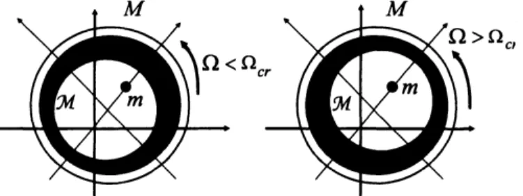
surface of the outermostwall, assketched in Fig. 1.

Consider the situation where an unbalancedmass $m$ is present, for exampledue tothe

non-uniform distribution ofclothes in a washing machine. The rotor has a critical angular velocity

$\Omega_{cr}$ where the centrifugal forces are in balance with the forces due to the restoring springs.

Belowthis velocity $(\Omega<\Omega_{cr})$ the

mass

center of the fluid will be located ‘on the

same

side’ as

the unbalanced mass, as shown in the left part of Fig. 1. [Here $M$ indicates the mass of the

$*a$_{[email protected],}$b$

empty rotor and $\mathcal{M}$the

mass

ofthecontained liquid.] At acertain supercritical angular velocity $\Omega>\Omega_{cr}$ (say, during the spin drying process) the

mass

center of the liquid will move to the

‘oppositeside’ ofthe unbalanced mass,

as

shown in the right part ofFig. 1, resulting in ‘mass

balance’ and thus in reduced centrifugal forces and reduced oscillation amplitudeof the rotor.

Figure 1: Workingprincipleof the fluid balancer.

This is the working principle of the fluid balancer. The main idea appeared already in

1912, and $US$ patent

was

granted in 1916 (Leblanc, 1916). The original layout consisted of

one or several very narrow concentric channels (narrow in the radial direction but wide in the

axial direction, i.e., perpendicular to the paper in Fig. 1) partially filled with, “liquid, or

very small steel balls ormetal fillings”. Leblanc’s fluid balancer

was

discussed and criticized by

Thearle (1932);and later also by Den Hartog(1985), inconnectionwith

a

discussion of Thearle’s

balancing head of 1932. It is argued there that Leblanc’s balancer cannot work with

a

liquid,

only withsteel balls, andthus that the invention

was

flawed. It appears that this is due to the

very narrow channels which basically prevent the formation ofsurfacewaves.

None the less, a complete automatic washing machine equipped with a fluid balancer was

presented in 1940, and patented in 1945 (Dyer, 1945). The layout of the fluid balancer

was

very

similarto themodern layouts, with awide concentric channel, wideenough to allow for surface

waveswith large amplitudes.

The idea is thus not new; but recently there has been a renewed interest, both in industry

and in academia. [There has also been a renewed interest in the so-called automatic dynamic

balancer,

as

the balancer that

uses

steel balls running in

a

circular channel (or race) is called

(vande Wouw et al., 2005; Green et al., 2006, 2008).$]$

Experimental fluid damper studies have been carried out by Kasahara et al. (2000a) and

Nakamura(2009). Astomathematicalmodels,simple lumpedmassmodelshavebeenconsidered

by Bae et al. (2002), Jung et al. (2008), Majewski (2010), Chen et al. (2011), and Urbiola-Soto

and Lopez-Parra (2011). The first andthelast two ofthesepapers include experimental studies

as well. The paper by Jung et al. (2008) includes a few numerical simulation results based on

computational fluid dynamics.

It should be emphasized that the fundamental principle of operation of the fluid balancer

can beunderstoodin termsof theexplanationof Thearle’s balancinghead, given inDen Hartog

(1985), p. 237. But a more detailed understanding is desirable; in particular, a more detailed

understandingof the fluid dynamics of the balancer.

the dynamics and stability of rotors partially filled with fluid/liquid; see e.g. Bolotin (1963)

and Crandall (1995) for good overviews. Most of the studies, such as those of Wolf, Jr. (1968),

Hendricks and Morton (1979) and Holm-Christensen and Tr\"ager (1991), are based on linear

theory/linearization. While this is sufficient to determine the stability properties, it may be

insufficient for modeling and understanding the dynamics of the fluid balancer (at any rate if

free (unforced) wave componentsare included) since the amplitudeof the surface

waves

needto

be known.

Non-linearstudies havebeencarriedout by Berman etal. (1985), Colding-Jrgensen (1991),

Kasahara et al. (2000b), and Yoshizumi (2007). Berman et al. (1985) found, both bynumerical

analysis and by experiment, that non-linear surface waves can exist on the fluid layer in the

formof hydraulic jumps, undularbores, and (what appears to be”) solitary waves (or solitons).

[An undular bore is a relatively weak hydraulic jump, with undulations behind it (Lighthill,

1978, p. 180). As to a solitary wave, described by the square of a hyperbolic secant function, sech, it should be noted that such a solution/wave exists only in a doubly infinite (i.e.

non-periodic) domain. In theperiodicdomainof the rotorvessel, thesolution whichcorresponds toa

solitarywaveis described bythe square ofa Jacobian elliptic cosine function, cn, and is termed

acnoidalwave.] Colding-Jrgensen(1991) concentrated onahydraulicjumpsolution, following

the analytical solution approach given in Berman et al. (1985). Contrary to this approach, the

studies of Kasahara et al. (2000b) and Yoshizumi (2007) are purely numerical.

As _{by Colding-Jrgensen (1991) the formulation of the basic shallow waterwavetheoryused}

inthe present paper is based largelyonthe approachof Berman et al. (1985). Thepresent work

considersarotorwith two degrees of freedom, contrary to the one-degree-of-freedomassumption

inBerman et al. (1985) and Colding-Jrgensen(1991). Also, rather than relyingona numerical

integration approach, we find an (approximate) analytical solution to the fluid equations via a

perturbation approach.

The presentpaper is to be considered

as

acontinuation of Langthjem and Nakamura (2011)

where the mathematical formulationofthe problem is described in detail.

2

The

fluid equations

and

approximate solution

of them

The fluid motion in the rotating vessel is described by a shallow water approximation of the

Navier-Stokes equations, and in terms of a coordinate system $(x, y)$ attached to the _{wall of the}

rotor. This coordinatesystemis relatedtoapolarcoordinate system $(r, \theta)$ attachedto the rotor

such that $x=R\theta,$

$y=R-r$

, where $R$ is the radius of the vessel. It is noted that _$x,$$y$ are

rectangular (Cartesian) coordinates, indicating that curvature effects will be ignored. This is permissable when the fluid layer thickness $h(t, x)$ is sufficiently small in comparison with the

vesselradius $R$, i.e., $|h(t, x)|/R\ll 1$ for all $x,$$t$

.

Under these assumptions the fluid equations of

motion can be written as (Berman et al., 1985; Whitham, 1999)

$\frac{\partial u}{\partial t}+u\frac{\partial u}{\partial x}+v\frac{\partial u}{\partial y}-2\Omega v = -\frac{1}{\rho}\frac{\partial p}{\partial x}+\nu\frac{\partial^{2}u}{\partial y^{2}}+\mathfrak{F}$, (1)

Here$u$ and $v$

are

thefluid velocity components in the $x$and $y$ directions,$p$is thefluid pressure, $\rho$ is the fluid density, $\nu$ is the kinematicviscosity ofthe fluid, and

$\mathfrak{F}$isa body force due to the

rotating vessel.

A perturbation approach applied to (1) and (2) gives the following equation for the

non-dimensional fluid layer perturbation $\kappa_{0}=h’/R$ (with $h’$ being the change in the fluid layer

thickness $h$):

$A_{1} \frac{\partial\kappa_{0}}{\partial\xi}-B_{1}\kappa_{0}\frac{\partial\kappa_{0}}{\partial\xi}-C_{1}\frac{\partial^{3}\kappa_{0}}{\partial\xi^{3}}-D_{1}\frac{\partial^{2}\kappa_{0}}{\partial\xi^{2}}+E_{1}\kappa_{0}^{2}=x_{*}\sin\xi-y_{*}\cos\xi$ , (3)

where $A_{1},$ $B_{1},$ $D_{1}$, and $E_{1}$ are parameters; see Langthjem and Nakamura (2011). The variable

$x_{*}$ and $y_{*}$ represent the vessel deflections, and $\xi$ is a ‘traveling wave’ variable, defined by $\xi=$ $\frac{x}{R}-(\omega-\Omega)t$. Here $\omega$is the angular whirling velocityofthevessel, which is assumed to beclose,

but not equal, to the imposed angular velocity $\Omega.$

Equation (3) isaforced Korteweg-de Vries-Burgersequation. Without damping$(D_{1}=E_{1}=$

$0)$ and external forcing $(x_{*}=y_{*}=0)$ it reduces to the classical Korteweg-de Vries equation.

The Burgers equation is obtained with $C_{1}=E_{1}=0$ (and again $x_{*}=y_{*}=0$ too). $A_{1}$ is

an

unknown parameter which can be determined from the condition that the fluid volume must

remain constant,

$\Delta V_{f}=\int_{0}^{2\pi}\kappa_{0}(\xi)d\xi=0$. (4)

2.1

Perturbation

solution of the

forced Korteweg-de

Vries-Burgers

equation

(3)

Viscous wallfrictionis ignored in the following; that is, in (3) it willbe assumed that$E_{1}=0$

.

The

effect of this term isnot uninteresting; but we are heremainly interestedjustin thequalitative

aspectsofthe fluid balancer dynamicsand wall friction is not considered to beessential in that respect.

When dividing through by$C_{1}$ (which is always $\neq 0$), (3) takes the form

$a_{1} \frac{\partial\kappa_{0}}{\partial\xi}-b_{1}\kappa_{0}\frac{\partial\kappa_{0}}{\partial\xi}-\frac{\partial^{3}\kappa_{0}}{\partial\xi^{3}}+\epsilon d_{1}\frac{\partial^{2}\kappa_{0}}{\partial\xi^{2}}=\epsilon(\hat{x}\sin\xi-\hat{y}\cos\xi)$ , (5)

where

$a_{1}= \frac{A_{1}}{C_{1}}, b_{1}=\frac{B_{1}}{C_{1}}, d_{1}=\frac{D_{1}}{C_{1}}$, (6)

and

$\hat{x}=\frac{x}{C_{1}}*, \hat{y}=\frac{y_{*}}{C_{1}}$

.

(7)

Here$\epsilon$ isa bookkeeping parameter’ (order symbol)whichisintroducedtoindicatethesmallness

of the rotor deflections $\hat{x},\hat{y}$

.

The damping parameter $d_{1}$ is assumed to be of the

same

order of

magnitude/smallness.

We seek anexpansion on theform

$\kappa_{0}(\xi)=v_{0}(\xi)+\epsilon v_{1}(\xi)+\cdots$ (8)

Atthe endof the analysis$\epsilon$ is set equaltoone. Itwill be

seen

that any term contained in $v_{1}(\xi)$

Inserting (8) int$o(5)$ we _get

$\epsilon^{0}$

order: $a_{1} \frac{\partial v_{0}}{\partial\xi}-b_{1}v_{0}\frac{\partial v_{0}}{\partial\xi}-\frac{\partial^{3}v_{0}}{\partial\xi^{3}}=0$, (9)

$\epsilon^{1}$ order:

$a_{1} \frac{\partial v_{1}}{\partial\xi}-b_{1}(v_{1}\frac{\partial v_{0}}{\partial\xi}+v_{0}\frac{\partial v_{1}}{\partial\xi})-\frac{\partial^{3}v_{1}}{\partial\xi^{3}}-d_{1}\frac{\partial^{2}v_{0}}{\partial\xi^{2}}=\hat{x}\sin\xi-\hat{y}\cos\xi$. (10)

2.2 Cnoidal

wave

solution of (9)

Equation (9) is a Korteweg-de Vries equation which can be solved in exact, closed form. The

solution is

$v_{0}(\xi)=\alpha cn^{2}[\Xi\xi, k]$

.

(11)

Here cn is the Jacobian elliptic cosine function (Whittaker andWatson, 1927; Abramomitz and

Stegun, 1965), withthe parameters

$\Xi=\{\frac{1}{12}b_{1}(2\alpha-3\frac{a_{1}}{b_{1}})\}^{\frac{1}{2}} k=\{\frac{\alpha}{2\alpha-3a_{1}/b_{1}}\}^{\frac{1}{2}}$ (12)

The solution (11) is called a cnoidal wave (due to the cn-function), and $\alpha$ is the amplitude of

thewave. The parameter $k$ is called the modulus (ofthe elliptic function).

The period of thefunctioncn$[\xi, k]$ is $4K$, where

$K=K(k)= \int_{0}^{\frac{\pi}{2}}(1-k^{2}\sin^{2}\theta)^{-\frac{1}{2}}d\theta$ (13)

is the complete elliptic integral of the first kind (Abramomitz and Stegun, 1965). Thus the period of$cn^{2}[\xi, k]$ is $2K$, and the period $(T_{0}, say)$ of the solution (11) is

$T_{0}= \underline{2K(k)}---=4K(k)\{\frac{3}{b_{1}(2\alpha-3a_{1}/b_{1})}\}^{\frac{1}{2}}$ (14)

We seeka$2\pi$-periodicsolution, such that $\kappa_{0}(0)=\kappa_{0}(2\pi)$. Thus,oneconditionfor determination

ofthetwo unknown parameters$\tilde{\omega}_{1}$ (which is hidden in

$a_{1}$) and $\alpha$ is that

$T_{0}(\tilde{\omega}_{1}, \alpha)=2\pi$, or $\triangle T_{0}=T_{0}(\tilde{\omega}_{1}, \alpha)-2\pi=0$

.

(15)

Another condition is that of conservation of fluid volume, asexpressed by (4).

It is noted, finally, that the Jacobian elliptic cosine function cn degenerates into the hyper-bolic secant function sech when $karrow 1$ and into the normal cosine function $\cos$ when $karrow 0.$

Regarding the first case, it will be

seen

from (13) that $karrow 1$ implies that the $Karrow\infty$, that is,

the period goes towards infinity. The solution in this case $(\alpha sech^{2}[\Xi\xi])$ is known as a solitary

wave, or asoliton.

2.3

Multiple scales solution of (10)

For the determination of $v_{1}(\xi)$, the second term in the expansion of $\kappa_{0}(\xi)$, we will make

the assumption that the modulus $k$ of $v_{0}(\xi)$ is small. The following expansion is then valid

(Abramomitz and Stegun, 1965):

Assuming here, forsimplicity, that $|k|\ll 1$,

we

dropthe $O(k^{2})$ terms. That is, forthe

determi-nation of$v_{1}(\xi)$, we

assume

that

$v_{0}( \xi)\approx\alpha\cos^{2}\Xi\xi=\frac{1}{2}\alpha\{1+\cos 2\Xi\xi\}$ . (17)

[It is noted here that in connection with the numerical examples to follow, it has beenverified

that $k$ actually is small.]

Now, integration of (10) with respect to $\xi$ gives

$a_{1}v_{1}-b_{1}v_{0}v_{1}- \frac{\partial^{2}v_{1}}{\partial\xi^{2}}-d_{1}\frac{\partial v_{0}}{\partial\xi}=-\hat{x}\cos\xi-\hat{y}\sin\xi+C_{1}$, (18)

where$C_{1}$ isan integration constant. We choose to set$C_{1}=0$ inorderto get aperiodic solution.

Inserting (17) into (18) gives, after reordering the terms,

$\frac{d^{2}v_{1}}{d\xi^{2}}+\{\mathfrak{a}^{2}+\frac{1}{2}\alpha b_{1}(1+\cos 2\Xi\xi)\}v_{1}=\hat{x}\cos\xi+\hat{y}\sin\xi+\alpha d_{1}\Xi\sin 2_{-}^{-}-\xi$, (19)

where $\mathfrak{a}^{2}$

is written in place $of-a_{1}$. [It is noted also that we write $dv_{1}/d\xi$ in place of$\partial v_{1}/\partial\xi$

from now on.]

Equation (19) isa forced Mathieuequation. Itis noted here that ifwe had used(11) directly

in (18) instead of the approximation (17), the homogeneous version of (19) would be a Lam\’e

equation. Exact solutions exist; these are termed Lam\’e functions and a considerable literature

about them exist $($Whittaker $and$ Watson, $1927; Ince, 1940a,b, 1956)$

.

Still, to solve the

non-homogenous Lam\’e equation, approximations (i.e., series expansions of Lam\’e functions) would

be necessary. It seems simpler, and in place, to introduce simplifications at anearlier

stage-already in the differential equation-as doneabove.

Now $\alpha$, which appears in (11), is used in the role of a small parameter. Employing the

method ofmultiplescales (Nayfeh, 2004), $v_{1}(\xi)$ is expanded

as

$v_{1}( \xi)=\sum_{m=0}^{M-1}\alpha^{m}\nu_{m}(\xi_{0}, \xi_{1}, \cdots, \xi_{M})$ , (20)

where

$\xi_{0}=\xi, \xi_{1}=\alpha\xi, \xi_{2}=\alpha^{2}\xi, \cdots$ (21)

It is notedthat, while the final solution (20) willcontain termsup to order$M-1$ ,the expansion must be carried out up to order $M$. We choose $M=2$; thus

$\frac{d\nu_{m}}{d\xi}=\frac{\partial\nu_{m}}{\partial\xi_{0}}+\alpha\frac{\partial\nu_{m}}{\partial\xi_{1}}+\alpha^{2}\frac{\partial\nu_{m}}{\partial\xi_{2}}=D_{0}\nu_{m}+\alpha D_{1}\nu_{m}+\alpha^{2}D_{2}\nu_{m}$ . (22)

Inserting (20) (running up to $M=2$) and (22) into (19) gives

$\epsilon^{0}$ order: $D_{0}^{2}\nu_{0}+\mathfrak{a}^{2}\nu_{0}=\hat{x}\cos\xi_{0}+\hat{y}\sin\xi_{0}$, (23)

$\epsilon^{1}$ order: _{$D_{0}^{2} \nu_{1}+\mathfrak{a}^{2}\nu_{1}=-2D_{0}D_{1}\nu_{0}-\frac{b_{1}}{2}(1+\cos 2_{-}^{-}-\xi_{0})\nu_{0}+d_{1}\Xi\sin 2\Xi\xi_{0}$} ,

(24)

$\epsilon^{2}$

The complete solutionto (23) is

$\nu_{0}(\xi_{0}, \xi_{1}, \xi_{2})=A(\xi_{1}, \xi_{2})e^{i\mathfrak{a}\xi_{0}}+\frac{1}{2}\frac{\hat{x}-i\hat{y}}{\mathfrak{a}^{2}-1}e^{i\xi_{0}}+c.c.$, (26)

where$A(\xi_{1}, \xi_{2})$ isacomplexfunction andc.c.denotes thecomplex conjugates of the preceeding

terms. Inserting (26) into (24) gives

$D_{0}^{2} \nu_{1}+\mathfrak{a}^{2}v_{1}=-e^{i\mathfrak{a}\xi_{0}}[2i\mathfrak{a}D_{1}A+\frac{b_{1}}{2}(1+\cos 2\Xi\xi_{0})A]-\frac{i}{2}d_{1}\Xi e^{i2\Xi\xi_{0}}$ (27)

$- \frac{b_{1}}{4}\frac{\hat{x}-i\hat{y}}{\mathfrak{a}^{2}-1}[e^{i\xi 0}+\frac{1}{2}e^{i(1+2\Xi)\xi_{0}}+\frac{1}{2}e^{i(1-2\Xi)\xi_{0}}]+c.c.$

Secular terms will not appear in the solution to (27) if

$2 i\mathfrak{a}D_{1}A+\frac{b_{1}}{2}(1+\cos 2\Xi\xi_{0})A=0$. (28)

Writing $A= \frac{1}{2}ae^{i\phi}$ and separating real and imaginaryparts gives

$\frac{da}{d\xi_{1}}=0, \frac{d\phi}{d\xi_{1}}=\frac{b_{1}}{4\mathfrak{a}}(1+\cos 2\Xi\xi_{0})$ . (29)

Theseequations have the solutions

$a= \hat{a}(\xi_{2}) , \phi=\frac{b_{1}}{4\mathfrak{a}}(1+\cos 2_{-}^{-}-\xi_{0})\xi_{1}+\hat{\phi}(\xi_{2})$ (30)

With (28) being satisfied, aparticular solution of (27) is

$v_{1}=- \frac{b_{1}}{4}\frac{\hat{x}-i\hat{y}}{\mathfrak{a}^{2}-1}[\frac{e^{i\xi_{0}}}{\mathfrak{a}^{2}-1}+\frac{e^{i(1+2_{-}^{--})\xi_{0}}}{2\{\mathfrak{a}^{2}-(1+2_{-}^{-}-)\}}+\frac{e^{i(-)\xi_{0}}1-2_{-}^{-}}{2\{\mathfrak{a}^{2}-(1-2_{-}^{-}-)\}}]$ (31)

$- \frac{i}{2}\frac{d_{1^{--}}^{-}-e^{i2-\xi_{0}}-}{\mathfrak{a}^{2}-4_{-}^{-2}-}+c.c.$

Next (26) and (31) areinserted into (25). This gives

$D_{0}^{2}v_{2}+ \mathfrak{a}^{2}v_{2}=[\frac{1}{2}\hat{a}(\xi_{2})(^{b}\lrcorner)^{2}(1+\cos 2\Xi\xi)^{2}-\mathfrak{a}\{i\frac{da}{d\xi_{2}}-\hat{a}\frac{d\phi}{d\xi_{2}}\}]\cross$ (32) $\cross\exp(i\mathfrak{a}\xi_{0})\exp(i(_{4\mathfrak{a}}^{b}\lrcorner)(1+\cos 2\Xi\xi_{0})\xi_{1}+\hat{\phi}(\xi_{2}))$

$+n.s.t. +c. c.,$

where n.s.t. stands for non-secular terms, that is, terms that arenot proportionalto $\exp(i\mathfrak{a}\xi_{0})$

.

Secularterms will not appear in the solutionto (32) if thetermsin the squarebracketsonthe

right-hand side are equal to zero. This condition gives, upon separation of real and imaginary

parts,

$\hat{a}(\xi_{2})=\overline{a}, \overline{\phi}(\xi_{2})=\frac{1}{2\mathfrak{a}}(\frac{b_{1}}{4\mathfrak{a}})^{2}(1+\cos 2\Xi\xi)^{2}\xi_{2}+\overline{\phi}$ , (33)

whereaand $\overline{\phi}$ areconstants. For the final

solution wewill choose$\overline{a}=0$ whichwill leave (11) as

the only free (unforced) waveoscillation component in thefinalsolution. Inserting these results

into (26) and (31) and returning to the original variableswe thus get

with

$\nu_{0}(\xi)=-\frac{1}{\mathfrak{a}^{2}-1}\{\hat{x}\cos\xi+\hat{y}\sin\xi\}$ (35)

and

$\nu_{1}(\xi)=-\frac{b_{1}}{2}\frac{1}{(\mathfrak{a}^{2}-1)^{2}}\{\hat{x}\cos\xi+\hat{y}\sin\xi\}-\frac{b_{1}}{4}\frac{\hat{x}\cos\{(1+2_{-}^{-}-)\xi\}+\hat{y}\sin\{(1+2_{-}^{-}-)\xi\}}{(\mathfrak{a}^{2}-1)\{\mathfrak{a}^{2}-(1+2_{-}^{-}-)^{2}\}}$ (36)

$- \frac{b_{1}}{4}\frac{\hat{x}\cos\{(1-2_{-}^{-}-)\xi\}+\hat{y}\sin\{(1-2_{-}^{-}-)\xi\}}{(\mathfrak{a}^{2}-1)\{\mathfrak{a}^{2}-(1-2_{-}^{-}-)^{2}\}}+\frac{d_{1-}^{-}-}{\mathfrak{a}^{2}-4_{-}^{-2}-}\sin 2\Xi\xi.$

Theresults given above

are

valid only when internal resonance does not take place, that is,

when $\mathfrak{a}^{2}$ is away

from 1. If $\mathfrak{a}^{2}$

is close to 1 then there

are

several special

cases

that need to

be analyzed, such

as

$\Xi$ close to 1, close to -, and $\Xi$ away from these values. In the numerical

work (to be described in the following) we have not experienced problemswith proximity to an

internal resonance. Accordingly thosespecial

cases

will not be analyzedhere.

3

Numerical evaluation

approach

There

are

four unknown parametersin ourproblem, namely afrequencyparameter$\tilde{\omega}_{1}$ included

in the coefficient $A_{1}$, the amplitude parameter $\alpha$defined by (11), and the rotor deflection

com-ponents $x_{*}$ and$y_{*}$. The four equations needed for determining these fourparameters are $(i, ii)$

the two coupled rotor equations ofmotion, (iii) thevolumeconstraint specified by (4), and (iv)

the periodicity constraint specified by (15). The unknown parameters are

now

determined

as

follows.

First guesses are made onthe values of$\tilde{\omega}_{1}$ and $\alpha$, in order to evaluate the fluid forces. [See

Langthjem and Nakamura (2011) forthe specific equations.] Thenthe rotorequation system is

solved with respect to $x_{*}$ and $y_{*}$

.

Following this, improved values of$\tilde{\omega}_{1}$ and $\alpha$

are

obtained by

taking one stepwith theNewton algorithm

$\{\begin{array}{l}\tilde{\omega}_{l}\alpha\end{array}\}=\{\begin{array}{l}\tilde{\omega}_{1}\alpha\end{array}\}-$$( \frac{1}{D}[-\frac{\partial\Delta V_{f}\Delta V_{f}\partial\alpha}{\partial\overline{\omega}_{1}}\frac{\partial}{}$ $- \frac{\partial\Delta To}{\partial\overline{\omega}_{1}\Delta T_{0}\partial\alpha}\frac{\partial}{}]\{\begin{array}{l}\tilde{\omega}_{1}\alpha\end{array}\})_{n}$ $D=| \frac{}{\partial\overline{\omega}_{1}}\frac{\partial\Delta T_{0}}{\partial\Delta\partial\overline{\omega}_{\star_{f}}}$ $\frac{}{\partial\alpha}\frac{\partial\Delta T_{0}}{\partial\Delta V_{f}\partial\alpha}|\cdot$ (37)

Then the fluid forces are again evaluated and the rotor equation system is again solved with respect to $x_{*}$ and $y_{*}$. This loop is continued until the absolute values of$\Delta V_{f}$ and $\Delta T_{0}$, which

should ideally be zero, are deemed sufficiently small, say smaller than $10^{-5}.$

4

Numerical

example

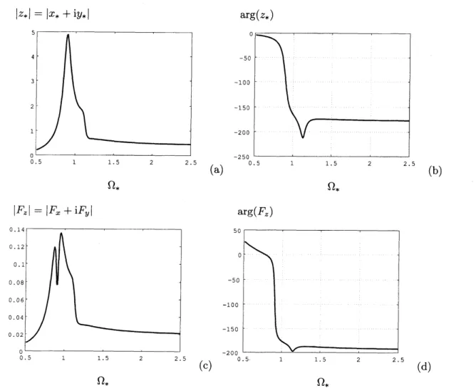
Vessel deflection components $x_{*},$ $y_{*}$ and fluid force components $F_{x},$ $F_{y}$ are shown in Fig. 2,

parts (a) and (c). Here $\Omega_{*}$ is anon-dimensionalvessel rotational speed, defined by $\Omega_{*}=\Omega/\omega_{S},$

with $\omega_{s}$ beingthe critical rotational speed for the empty rotor.

Part (b) and (d) show the phase angle of the vessel deflection $(\varphi_{d}, say)$ and ofthe resultant

fluid force $(\varphi_{f}, say)$, respectively. The phase angle of the deflection starts, by small rotational

speeds, at$\varphi_{d}\approx 0$; that is, thedeflectionisin thedirectionof the unbalanced

mass.

Uponpassing

throughresonance thephase angle shifts approximately $180^{o}$

.

(Byzooming inonthe graphthe

precisevalue $\varphi_{d}=-177^{0}$isfound.) The phase angleof the resultant fluid force (shown byafull

$|z_{*}|=|x_{*}+iy_{*}|$ $\arg(z_{*})$ (a) (b)

$\Omega_{*} \Omega_{*}$

$|F_{z}|=|F_{x}+iF_{y}|$ $\arg(F_{z})$ (c) (d)

$\Omega_{*} \Omega_{*}$

Figure 2: Vessel deflection and fluid force amplitudes $(a, c)$ and phase angles $(b, d; in$ _degrees)

as functions ofthe angular velocity $\Omega_{*}.$

Thus, after thepassagethroughresonance, the resultantfluidforcestarts to work against the

unbalanced mass, tendingto generate a deflection which is opposed tothe deflection generated

by the unbalanced mass. This explains the basic dynamics ofthe fluid balancer.

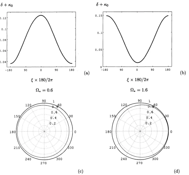
Fig. 3 shows the liquid surface, described by the non-dimensional parameters $\delta+\kappa_{0}$, fora

sub-criticalvalue of$\Omega_{*}(\Omega_{*}=0.6)$inparts (a) and (c); and forasuper-criticalvalue_{$(\Omega_{*}=1.6)$}in

parts (b) and(d). [Parts (a) and (b) givean‘outfolded’representationin rectangular coordinates,

while parts (c) and (d) give a more physical representationin polar coordinates.]

It is noted that ‘unphysical’ solutions can be generated around $\Omega_{*}\approx 1$, in the sense that

$\delta+\kappa_{0}(\xi)$ (which should be $>0$ for all $\xi$) can become $<0$ at certain values of$\xi$. The problem has been reported and discussed also by Jung et al. (2008) and Urbiola-Soto and Lopez-Parra

(2011). In order to avoid it, constraints on the form $\delta+\kappa_{0}(\xi)>0$ should be imposed at a

relatively large number of values of$\xi$ around the circumference. This will implythat there will be (many) moreequationsthan unknowns andwillin turnrequirethat the Newton method (37) is replaced by, for example, a least squares methodology. We prefer, however, to avoid this at

thepresent stage. The issue does not cause any ‘singular’ behavior in the equation system and

Retuming to Fig. 3, initially $(at time t_{*}=0, say)$ the unbalanced

mass

is located at $\xi=0,$

in a coordinate system moving with the whirl (i.e., with the angular velocity $\omega-\Omega$, or $\tilde{\omega}-1$

in terms of non-dimensional parameters). Thus, a wave top is located at the position of the

unbalanced

mass

by the sub-critical rotational speed, and opposite of the unbalanced

mass

by

thesuper-critical rotational speed, just

as

illustrated in Fig. 1. There is however a slow drift’

withangularvelocity $1-\tilde{\omega}$

.

Thisundesirable phenomenon has been verified inexperiments, and

various remedies have been considered in order to prevent it, e.g. a hexagon-shaped channel

and separator plates (Nakamura, 2009).

$\delta+\kappa_{0}$ $\delta+\kappa_{0}$

$-180$ 90 $0$ 90 180

(a) (b)

$\xi\cross 180/2\pi \xi\cross 180/2\pi$

$\Omega_{*}=0.6 \Omega_{*}=1.6$

$270 270$

(c) (d)

Figure 3: The fluidlayer in thevessel, described by$\delta+\kappa_{0}$, in terms of‘rectangular’ plots (a, b)

and polar plots (c, d). The unbalanced

mass

is initially $(at time t_{*}=0, say)$ located at $\xi=0.$

Parts (a) and (c) show the fluid layer before

resonance

$(\Omega_{*}=0.6)$ and parts (b) and (d) the

5

Conclusion

The dynamics of the fluid balancer has been investigated basedon a modelofatwo

degrees-of-freedom rotor containing asmallamount ofliquid. The thininternalfluidlayer,which forms due

tothe rotation,is describedinterms of shallowwaterwavetheory. $A$perturbation approachgives

that the fluid layer thickness perturbation is described by a forced Korteweg-de Vries-Burgers

equation. This equation_{is solved- approximately-also by a perturbation approach. The first} approximationinvolves$a$ (single) cnoidalwavesolution of the (homogeneous) Korteweg-de Vries

equation. The next term in the approximationis govemed bya forced Mathieu equation. The fluid and rotor equations are coupled by integrating the fluid pressure over the inner

vesselsurface. The phase anglefunctionofthe resultant fluidforcehasa behaviorthatresembles

theexperimentallyobtained function (Nakamura, 2009). In particular, it isconfirmed that,when

the unbalanced

mass

initially is placed at the angular position $\varphi=0$ (in

a

coordinate system

moving with the whirl), the phase angle of the resultant fluid force moves from $\varphi=0^{o}$ at

subcritical rotational speeds to $\varphi=180^{0}$ at supercritical speeds; that is, after passage through

resonance. As observed in experiments, there is however a drift of the resultant fluidforce.

Finally,itmustbe mentioned that it is notdifficulttofind parameter values where thepresent

numerical approach does not convergence. This suggests that a stable

one-wave

solution does

not exist (at those parameter values). Numerical simulations $($Kasahara $et al., 2000b)$ suggest

the existence of multi-wave solutions, stillof solitary (or rather, cnoidal) wave type. It is known

(Miura, 1976) that the Korteweg de-Vries equation (9) admits multiple-soliton solutions (in a

doubly infinite domain). It would be interestingto pursue such analytical multi-wave solutions

to the fluid balancerproblem in future research.

References

Abramomitz, M. and Stegun, I. A. (1965). Handbook

_of

Mathematical Functions. Dover

Publi-cations, Inc., New York.

Bae, S., Lee, J. M., Kang, Y. J., Kang, J. S.) and Yun, J. R. (2002). Dynamic analysis ofan

automatic washing machine with a hydraulic balancer. J. Sound Vib., 257, 3-18.

Berman, A. $S$., Lundgren, T. $S$., and Cheng, A. (1985). Asyncronouswhirl inarotating cylinder

partiallyfilled with liquid. J. Fluid Mech., 150, 311-327.

Bolotin, V. $V$. (1963). Nonconservative Problems

of

the Theory

of

_{Elastic Stability. Pergamon}

Press, Oxford, $UK.$

Chen, H.-$W$., Zhang, Q., and Fan, S.-$Y$

.

(2011). Studyonsteady-stateresponse ofavertical axis

automatic washing machine with a hydraulic balancer using a new approach and a method

forgetting asmaller deflectionangle. J. Sound Vib., 330, 2017-2030.

Colding-Jrgensen, J. (1991). Limit cycle vibration analysis ofa long rotating cylinder partly

Crandall, S. $H$

.

(1995). Rotor dynamics. In W. Kliemann and N. S. Namachivaya, editors,

NonlinearDynamics and Stochastic Mechanics, pages 1-44. CRC Press, Boca Raton.

Den Hartog, J. $P$

.

(1985). Mechanical Vibrations. Dover Publications, Inc. [Orig. 4th Ed. by

McGraw-Hi111956], New York.

Dyer, J. $B$

.

(1945). Domestic appliance. U. S. Patent No. 2,375,635.

Green, K., Champneys, A. $R$., and Lieven, N. $J$

.

(2006). Bifurcation analysis of an automatic

dynamic balancing mechanism for eccentric rotors. J. Sound Vib., 291, 861-881.

Green, K., Champneys, A. $R$., Friswell, M. $I$., and Munoz, A. $M$

.

(2008). Investigation of

a

multi-ball, automatic dynamic ballbalancing mechanism for eccentric rotors. Phil. Trans. $R.$

Soc. $A,$ $366,705-728.$

Hendricks, S. $L$

.

and Morton, J. $B$

.

(1979). Stability of a rotor partially filled with a viscous

incompressiblefluid. J. Appl. Mech., 46, 913-918.

Holm-Christensen, O. and Tr\"ager, K. (1991). $A$ note on rotor instability caused by liquid

motions. J. Appl. Mech., 58, 804-811.

Ince, E. $L$. (1940a).

.The

periodic Lam\’efunctions. Proc. _$Roy$

.

Soc. Edinburgh, 60,

47-63.

Ince, E. $L$

.

(1940b).

2Further

investigations into the periodic Lam\’e functions. Proc. $Roy$

.

Soc.

Edinburgh, 60, 83-99.

Ince, E. $L$

.

(1956). Ordinary

Differential

Equations. Dover Publications, Inc., New York.

Jung, C.-$H$., Kim, C.-$S$., and Choi, Y.-$H$

.

(2008). $A$ dynamic model and numerical study

on

the

liquid balancer used in an automatic washing machine. J. Mech. Sci. Tech., 22,

1843-1852.

Kasahara, M., Kaneko, S., Oshita, K., and Ishii, H. (2000a). Experiments ofliquidmotion in a

whirling ring. In Proceedings

of

the Dynamics and Design

_Conference

2000, 5-8August 2000,

pages 1-6, Tokyo, Japan. Japan Soc. Mech. Eng.

Kasahara, M., Kaneko, S., and Ishii, H. (2000b). Sloshing analysis of

a

whirling ring. In

Proceedings

_of

theDynamics and Design

_Conference

2000, 5-8August 2000, pages1-6, Tokyo,

Japan. Japan Soc. Mech. Eng.

Langthjem, M. $A$. andNakamura, T. (2011). Dynamics ofthefluid balancer. RIMSKokyoroku,

1761, 140-150.

Leblanc, M. (1916). Automatic balancer for rotating bodies. U. S. Patent No. 1,209,730.

Lighthill, J. (1978). Waves in Fluids. Cambridge University Press, Cambridge, $UK.$

Majewski, T. (2010). Fluid balancer fora washingmachine. In Proceedings

_of

the XVI

Intema-tional Congress, pages 1-10. SOMIM (Societyof Mechanical Engineers ofMexico).

Miura, R. $M$

.

(1976). The Korteweg-de Vries equation: $A$ survey of results. SIAMReview, _$1S,$

Nakamura, T. (2009). Study ontheimprovement of the fluid balancerof washing machines. In

Proceedings

_of

the 13th

_Asia-Pacific

Vibrations Conference, 22-25 November 2009, pages1-8.

University ofCanterbury, New Zealand.

Nayfeh, A. $H$

.

(2004). Perturbation Methods. Wiley-VCH Verlag, Weinheim.

Thearle, E. (1932). $A$new type of dynamic-balancing machine. Trans. ASME, 54, 131-141.

Urbiola-Soto, L. andLopez-Parra, M. (2011). Dynamic performanceof the Leblanc balancerfor

automatic washing machines. J. Vibr. Acoust., 133,

041014-1-041014-8.

vandeWouw, N.,vanden Heuvel, M.$N$., Nijmeijer, H., andvanRooij,J.$A$. (2005). Performance

ofan automatic ball balancer with dry friction. Int. J.

_Bifurcation

and Chaos, 15, 65-82.

Whitham, G. $B$

.

(1999). Linear and Nonlinear Waves. Wiley-Interscience, New York.

Whittaker, E. $T$

.

and Watson, G. $N$

.

(1927). A Course

of

Modern Analysis. Cambridge

Univer-sity Press, Cambridge, $UK.$

Wolf, Jr., J. $A$. (1968). Whirl dynamics of a rotor partially filled _{with liquid. J.} Appl. _Mech.,

35, 676-682.

Yoshizumi, F. (2007). Self-excited vibration analysis of a rotating cylinder partiall filled with

liquid (Nonlinear analysis by shallow watertheory). Trans. Japan Society

_of

Mech. $Eng.$ $(C)$,