Periodic Solutions of the Forced Burgers Equation (Mathematical Analysis in Fluid and Gas Dynamics)

Periodic Solutions

of the Forced Burgers

Equation

1

Problem

We consider the forced Burgers equation

早稲田大学

(Waseda University)

西田孝明

(Takaaki Nishida)

[email protected]

早稲田大学

(Waseda

University)

曽我幸平

(Kohei Soga)

[email protected]

(1.1) $u_{t}(x, t)+u(x, t)u_{x}(x, t)=F_{x}(x, t)$_,

where the forcing term $F_{x}$ is the partial derivative of

a

given $C^{2}$

-function

_$F$ which

is periodic in both $x$ and $t$ with the period 1. The problem is to find $\mathbb{Z}^{2}$-periodic

(weak) solutions _{of (1.1), namely periodic solutions with the period 1 in both} $x$ and $t$,

in constructive ways. Our basic tool is the Lax-Friedrichs difference scheme. We present

two methods of constructing $\mathbb{Z}^{2}$-periodic

solutions of (1.1): Tlie one is based on the long

time behavior of the Lax-IFlriedrichs difference scheme. The other is based

on

Newton’s

method, regarding$\mathbb{Z}^{2}$-periodic

solutions

as

fixed

pointsof thePoincar\’e

map

derived from

the $Lax- Riedric\cdot hs$ scheme. We give

convergence

_{proofs to these methods and simulate} $\mathbb{Z}^{2}$

-periodic solutions.

It is _{known that there is}

_an

_{interesting connection between the forced Burgers}

equa-tion and Hamiltonian dynamics. One of the central issues in the theory ofHamiltonian

dynamics is to look for their invariant manifolds. The graph of

a

$\mathbb{Z}^{2}$

-periodic

solu-tion to (1.1) plays

an

important role in the issue. We also simulate trajectories of the

Hamiltonian dynamics corresponding to the forced Burgers equation and $vis^{\backslash }ualize$ their

connection.

2

Background

In this section

we

state the history of

our

problem. Let

us

go

back

to

Boltzmann’s

statistical mechanics.

Boltzmann

tried to derive thermodynamics from the dynamics of

particles. The dynamics of particles is governed by Hamiltonian systems

(2.1) $x’(s)=\mathcal{H}_{y}(x(s), y(s))$, $y’(s)=-\mathcal{H}_{x}(x(s), y(s))$,

where the

Hamiltonian

$\mathcal{H}(x, y)$ : $\mathbb{R}^{2n}arrow \mathbb{R}$ is the total energy of particles. Because

of the energy _{conservation law, each trajectory} $(x(\backslash 9), y(s))$ of (2.1) is trapped

on

the

$2n-1$-dimensional energy level set

In

order

to

derive

thermodynamical variables such $u$ entropy, temperature, pressure,

etc., it is required that

for

each

function

$G(x, y)$ the following equality

holds:

$<$ time-average

of

$G$ along any trajectory

on

$\Sigma_{h}>=$ $<$ space-average

of

$G$

on

$\Sigma_{h}>$

.

This is possible, if each trajectory on $\Sigma_{h}$ passes through all the points

of

$\Sigma_{h}$ (Boltzmann’s

ergodic hypothesis). After this hypothesis was presented, many mathematicians started

to analyze the ergodic problems and improved Boltzmann’s ergodic hypothesis (see [4]),

Although $tI_{1}e$ consequences of tlie ergodic properties of the equations (2.1)

come

out,

it is not easy to find Hamiltonian systems with the ergodic properties. As

an

example,

let us consider harmonic lattices, which

are a

model of crystals. In the

case

of the

l-dimensional harmonic lattice with fixed end points, its total energy is given by

(2.2) $\mathcal{H}(x, y)=\sum_{i=1}^{r\iota}\frac{1}{2}y_{i}^{2}+\frac{1}{2}\kappa^{i}x_{1}^{2}+\sum_{i=1}^{n-1}\frac{1}{2}\kappa(x_{i+1}-x_{i})^{2}+\frac{1}{2}\kappa^{r}x_{r\iota}^{2}’$.

We

can

find $t\mathfrak{l}_{1}e$ symplectic transform: $(x, y)\mapsto(\tilde{x},\tilde{y})w1\downarrow ic\cdot\}_{1}$ decornposes the motions of

the system (2.1) into the normalmodes. The

new

Hamiltonian $\tilde{\mathcal{H}}$

takes the simpler form

$\tilde{\mathcal{H}}(\tilde{x},\tilde{y})=\sum_{i=1}^{r}\frac{1}{2}\omega_{i}(\tilde{x}_{i}^{2}+\tilde{y}_{i}^{2})$ ($\omega=(\omega_{1},$ $\cdots,$$\omega_{n})$ is constant).

By the symplectic polar coordinates $(q,p)\in T^{n}\cross(\mathbb{R}_{+})^{n},$ $T^{n}:=\mathbb{R}^{n}/2\pi \mathbb{Z}^{n}$ defined by

$\tilde{x}_{i}=\sqrt{2p_{i}}\sin q_{i}$, $\tilde{y}_{i}=\sqrt{2p_{i}}\cos q_{i}$,

$\tilde{\mathcal{H}}$

changes into

$H(q,p)= \sum_{i=1}^{n}\omega_{i}p_{i}:T^{n}\cross(\mathbb{R}_{+})^{n}arrow \mathbb{R}$.

Therefore each trajectory is given by

$(q(s),p(s))=(\omega s+q(O),p(O))$ niod $2\pi$,

which implies for any $s\in \mathbb{R}$

$(q(s),p(s))\in \mathcal{I}:=T^{n}\cross\{p(0)\}$.

$Eac\cdot I\iota$ trajectory is _$traI$)$ped$ on an $r\iota$

-dirnensional

torus and cannot be ergodic!

Fermi, Pasta and Ulam [2] made numerical siniulatioiis to anharmonic lattices which

have non-quadratic potential energy in addition to (2.2). In the anharmonic cases, the

above reduction yields the Hamiltonian of the form

$H(q,p)= \sum_{i=1}^{n}\omega_{i}p_{i}+H_{1}(q,p):T^{n}\cross(\mathbb{R}_{+})^{n}arrow \mathbb{R}$,

where $H_{1}$ is a perturbation due to the anharmonic potential

energy.

Since $H_{1}$ depends

on

$q$, it is difficult to give expression of each trajectory $(q(s),p(s))$

.

They expected

results, however, suggested strongly that $7nar\iota y$ trajectories

of

anharmonic lattices are

still trapped on slightly

_deformed

n-dimensional

tori and not ergodic.

Nishida [7] showedthat the $KAM$theory, _{stated later, is applicabletothe anharmonic}

lattices and proved that there exist the

_deformed

n-dimensionaltori

on

which trajectories

are

trapped.

Existence of such deformed n-dirnensional tori is significant to an understanding of

the stability or instability of

Hamiltonian

dynamics. Now

we

give a brief description of

the problem of the search for such deformed n-dimensional tori.

We consider $C^{2}$

-Hamiltonians

(2.3) $H(q,p):T^{r\iota}\cross Darrow \mathbb{R},$ $T^{n}:=\mathbb{R}^{n}/\mathbb{Z}^{n},$ $D\subset \mathbb{R}^{n}$

and

Hamiltonian

systerns

(2.4) $q’(s)=H_{p}(q(s)\}p(s))$_{, $p’(s)=-H_{q}(q(s),p(s))$}

.

The solution (trajectory) of (2.4) with

an

initial value $(\theta, I)\in T^{n}\cross D$ is

denoted

by

$\phi_{H}^{s}(\theta, I)$,

where $\phi_{H}^{s}$ is the flow of (2.4). A manifold $\mathcal{I}$is called

a

$\phi_{H}^{S}$-invariant

manifold

diffeomor-phic to $T^{n}$

or

just

$\phi_{H}^{s}$-invariant $n$-torws, if $\mathcal{I}$ is

an

ernbedded

$n$-dimensional torus by

a

smooth embedding: $T^{n}arrow T^{n}\cross D$ and satisfies for each $s$

$\phi_{H}^{s}(\mathcal{I})\subset \mathcal{I}$

.

First,

we

consider the simple

case

where Hamiltonians

are

of the form

$H(q,p)=H_{0}(p)$

.

It is proved that, in “general”, Hamiltonians of integrable Hamiltonian systems

_can

be

brought intothe

above

form by

an

appropriate symplectic transform (e.g.,

see

[6]). The

harmonic lattice is an example of integrable Hamiltonian systems. Each trajectory is

represented by

$\phi_{H}^{s}(\theta, I)=(\partial_{p}H_{0}(I)s+\theta,$ $I)mod 1$,

where $\partial_{p}H_{0}$ is thegradient of$H_{0}$.

Hence we can

find $\phi_{H}^{s}$-invariant n-torus for each $I\in D$

$\mathcal{I}:=T^{n}\cross\{I\}$,

which implies that the phase space $T^{n}\cross D$ is foliated by these tori, namely

$T^{n}\cross D=\cup \mathcal{I}$

.

Each $\mathcal{I}$ carries trajectories

$(q(s), p(s))$, which

are

just straight lines with the

same

slope

$\lambda:=\lim_{|s|arrow\infty}\frac{\tilde{q}(s)}{s}=’\partial_{p}H_{0}(I)$,

where $q(s)=\tilde{q}(s)mod 1$. $\lambda$ is called the frequency vector of the

Next

we

consider the perturbed Hairiiltonians

$(2_{\iota}^{r}))$ $H(q,p)=H_{0}(p)+H_{1}(q,p)$ : $T^{n}\cross Darrow \mathbb{R}$,

where $H_{1}$ is

a

perturbation. Because of the so-called small divisor problem, people had

difficulties in proving existence of $\phi_{H}^{\theta}$-invariant $r\iota$-tori for (2.5). In 1954, Kolmogorov

brouglit the great progress. His arguments

were

completed byArnoldarid Moser, whichis

now

well-known

as

theKAM theory. Oneof the main assertion ofthe KAMtheory isthat

there exist the $\phi_{H}^{s}$-invariant n-tori carrying trajectories with the strongly nonresonant

frequency vectors:

The KAM

Theorem

([5][1]).

Let

$D$ be

a bounded

connected closed domain

of

$\mathbb{R}^{n}$

.

Suppose $(A 1)-(A3).\cdot$

$(A1)H(q, p)=H_{0}(p)+H_{1}(q,p)$ is analytic $or\iota$ a complex neighborhood $G$

of

$T^{n}\cross D$,

$(A2)H_{0}$ is nondegenerate, namely the Hessian matrix

of

$H_{0}$ has rank $n$

on

$D$,

(A3) $\Vert H_{1}\Vert=\sup_{G}|H_{1}(q,p)|$ is sufficiently small.

Then there exists afamily

_of

$KAM$n-tori $\mathcal{I}wf\iota ose$ union

satisfies

thefollowing

measure

estimate:

mes$[\cup \mathcal{I}]arrow$

mes

$[T^{n}\cross D]$ as

1

$H_{1}\Vertarrow 0$,

where

a

$KAM$ n-torus $\mathcal{I}$ is a

$\phi_{H}^{8}$-invariant

manifold

diffeomorphic to $T^{n}$ which is a

Lagrangian

_sub-manifold

and

$ca$rries quasi-periodic trajectories with the

same

frequency

vector $\lambda$ satisfying the Diophantine condition.

The developments of the

KAM

theory within half

a

century

are

collected in [9]. The

KAM

theory leaves interesting questions: What is going on in the region $I^{n}\cross D\backslash \cup \mathcal{I}$?

What happens for large perturbations? Nurnerical studies tell

us

that tliere

are

irregular

trajectories called “chaos”, which sometimes

seem

to be ergodic in Boltzmann’s

sense.

Finally

we

search for $\phi_{H}^{\delta}$-invariant n-tori in the general

case

with $C^{2}$-Hamiltonians

(2.3). We restrict ourselves to the manifolds diffeomorphic to $\nu_{J1^{n}}$ which

are

of the form

(2.6) $\{(q, \partial S(q))|q\in T^{r\downarrow}\}$,

where $S$ : $\mathbb{R}^{n}arrow \mathbb{R}$ is

a

$C^{2}$-function with the $\mathbb{Z}^{n}$-periodic gradient $\partial S$

.

Note that they

are

Lagrangian sub-manifolds. It is easily proved that each KAM n-torus takes the form

(2.6) with

a

real analytic function $S$ satisfying the Hamilton-Jacobi equation

(2.7) $H(q, \partial S(q))=h$ in $\mathbb{R}^{n}$ ($h$ is constant)

with the real analytic Hamiltonian $H(q,p)=H_{0}(p)+H_{1}(q,p)$

.

Let

us

consider the

Hamilton-Jacobi equations (2.7) with general $C^{2}$-Hamiltonians. Note that each solution

of the

Hariiiltoniari

system (2.4) is part of the

characteristics

of (2.7). The following

assertion is well-known: Let $H$ : $T^{n}\cross Darrow \mathbb{R}$ and $S:\mathbb{R}^{n}arrow \mathbb{R}$ be a $C^{2}$

-function.

Then

the graph

_of

$\partial S(q)$

$\mathcal{I}_{\partial S}:=\{(q, \partial S(q))|q\in T^{n}\}$

is

a

$\phi_{H}^{S}$-invariant

manifold

diffeomorphic to $\mathbb{T}^{n}$,

if

and only

_if

$S$ is

a

$C^{2}$-solution

of

have the following: Let $S$ be a $C^{2}$-solution

of

the

Hamilton-Jacobi

equation $(6l.7)$ with

the $\mathbb{Z}^{n}$-periodic gradient

$\partial S(q)$

.

If

$n=2$ and $H$

satisfies

the relation $H(q_{1}, q_{2_{7}}p_{1},p_{2})=h\Leftrightarrow p_{2}=f(q_{1)}q_{2},p_{1};h)$,

then $u(q)$ $:=S_{q_{1}}(q)$ is a $\mathbb{Z}^{2}$-periodic _$C^{1}$

-solution

_of

the scalar conservation law

(2.8) $\partial_{q_{2}}’u(’.q_{1}, q_{2}, u(q_{1}, q_{2}’))\}$ in $\mathbb{R}^{2}$

and the graph$\mathcal{I}_{\partial S}$ is represented by

$\mathcal{I}_{\partial S}=\{(q, u(q), f(q, u(q);h))|q\in T^{2}\}$

.

A $C^{1}$-solution of (2.8) yields a $C^{2}$-solution ofthe corresponding

Hamilton-Jacobi

equa-tion. Of

course

we

cannot always expect classical

solutions

of the

Hamilton-Jacobi

equations (2.7)

or

tfie scalar conservation laws (2.8). This implies that we may have no

universal methods

_of

searching

_for

the $\phi_{H}^{s}$-invariant

n-tore

we

are

concemed with,

even

no

such tori.

An interesting question arises: what is the relation among regular/chaotic properties

of

the Hamiltonian systems (2.4), viscosity solutions

_of

the Hamilton-Jacobi equations

(2.7) and entropy solutions

_of

the scalar conservation laws (2.8).

We consider this question taking

a

simple example of

a

nonlinear pendulum in the

extended phase space with the

Hamiltonian

of the

form

(2.9) $H(q_{1}, q_{2},p_{1},p_{2})= \frac{1}{2}p_{1}^{2}+p_{2}-F(q_{1}, q_{2}):T^{2}\cross \mathbb{R}^{2}arrow \mathbb{R}$

.

We

assume

that $F$ is a $C^{2}$-function. The corresponding scalar conservation law (2.8)

becomes the

forced

Burgers equation (1.1):

$u_{t}(x, t)+u(x, t)u_{x}(x, t)=F_{x}(x, t)$,

replacing the variables $(q_{1}, q_{2})$ with _{$(x, t)$}

.

The Hamiltonian system for (2.9) is reduced

to the nonautonomous

Hamiltonian

system

(2.10) $X’(s)=U(s)$, $U’(s)=F_{x}(X(s), s)$,

whichgivesthe

characteristics

of (1.1). We focus

our

attentiononthe connectionbetween

$\mathbb{Z}^{2}$

-periodic entropy solutions of (1.1) and the dynamics of (2.10).

Jauslin, Kreiss and Moser [3] obtained $\mathbb{Z}^{2}$

-periodic solutions of (1.1) by the vanishing

viscosity method. They also pointed out several interesting open problems

on

the forced

Burgers equation and the corresponding Hamiltonian dynamics. They considered the

parabolic equations with the periodic boundary condition

(2.11) $u_{t}^{\nu}(x, t)+u^{\nu}(x, t)u_{x}^{\nu}(x, t)=F_{x}(x, t)+\nu u_{xx}^{\nu}(x, t)$ in $T\cross \mathbb{R}_{+}$,

where $\nu>0$ is an artificial _{viscosity. Using the long time behavior ofsolutions to (2.11),}

they proved the following: For each $\nu>0$ and $C\in \mathbb{R}$ there exists the unique $\mathbb{Z}$-periodic

in $t$ solution$\overline{u}^{\nu}\in C^{2}$ to (2.11) such that

for

all $t\in \mathbb{R}$

Moreover there is a sequence

$\overline{u}^{1}$ノ

$t\in\{\overline{u}^{\nu}|\nu>0, <\overline{u}^{\nu}>=C\}$

with $\nu_{i}arrow 0$ which converges to a $\mathbb{Z}^{2}$-penodic entropy solution $\overline{\iota\nu}$

of

(1.1) $with<\overline{u}>=C$

in the $C^{0}(T;L^{1}(T))$-topology.

Takeno [10] also obtained $\mathbb{Z}^{2}$-periodic solutions of

(1.1) by the Lax-Friedrichs

differ-ence

scheme and Brouwer’s fixed point theorem. He regarded approximate $\mathbb{Z}^{2}$-periodic

solutions of (1.1)

as

fixed points of the Poincar\’e map derived from the Lax-Friedrichs

difference scheme and showed existence of these fixed points by Brouwer’s fixed point

theorem.

$E[11]$ _{made clear the connection} between $\mathbb{Z}^{2}$-periodic solutions of (1.1)

and

regular

motions of the corresponding Hamiltonian system. His results include

a

_flow

version

_of

the Aubry-Mather theory

_for

twist maps. Let $\overline{u}$ be a$\mathbb{Z}^{2}$-periodic

entropy solution of (1.1)

with $<\overline{u}>=C$ and $c(s)$ $:=(\tilde{X}(s), s, U(s))mod 1$ _{be characteristic}

curves

_{derived from}

the equations (2.10). He proved the following: Each characteristic

curve

$c(s)$ which is

defined

on

$(-\infty, \tau]$ with $\tau\in[0,1]$ and

satisfies

the initial condition

$c(\tau)\in graph(\overline{u})$ $:=\{(x, t,\overline{u}(x, t))|(x, t)\in T^{2}\}$

is trapped

on

graph$(\overline{u})$ and never absorbed by the shocks

of

$\overline{u}$

.

The motion

of

$c(s)$ on

graph$(\overline{u})$ is characterized by the asymptotic slope

$s arrow-\infty 1i_{IIl}\frac{\tilde{X}(s)}{s}=\alpha(C)$,

where $\alpha(C)$ depends only on the average

C.

Moreover there exist charactertstic

curves

$c^{*}(s)=(\tilde{X}^{*}(s), s, U^{*}(s))mod 1$

defined

on

$\mathbb{R}$ with the

same

asymptotic slope

$\lim_{|s|arrow\infty}\frac{\tilde{X}^{*}(s)}{6}=\alpha(C)$

which are trapped

on

$gr\cdot apf\iota(\overline{u})$ and

never

$absor\cdot bed$ by the shocks. For any given $\alpha\in \mathbb{R}$

there exists $C\in \mathbb{R}$ such that $\alpha(C)=\alpha$. Note that if $\overline{u}$ is a $C^{1}$-function, then any $c(s)$

with an initial condition on graph$(\overline{u})$ is trapped on it for any $s\in \mathbb{R}$. In the original

$pha\backslash e$space $T^{\prime z}\cross D$ with the Hamiltonian (2.9), these results

mean

that for each $h\in \mathbb{R}$

the set

$\mathcal{I}_{\overline{u}}:=\{(q,\overline{u}(q), h-\frac{1}{2}\overline{u}(q)^{2}+F(q))|q\in T^{2}\}$

is $\phi_{H}^{s}$-backward-invariant. Moreover there exists a $\phi_{H}^{S}$-invariant closed set $\Gamma^{*}\subset \mathcal{I}_{\overline{u}}$, on

which each trajectory has the frequency vector

$\lambda=(\alpha(C), 1)$.

Note that if $\overline{u}$ is

a

$C^{1}$-function, then $\mathcal{I}_{\overline{u}}$ is

a

$\phi_{H}^{S}$-invariant manifold diffeomorphic to $T^{2}$.

3

Main Results

Analytical results. We make

use

ofthe two-step $Lax- R\dot{n}edr\dot{v}chs$

difference

scheme on

$T\cross \mathbb{R}_{\geq 0}\ni(x, t)$: Let $N,$ $K$ be natural numbers. We define the mesh sizes

as

We set $x_{n};=r\iota\Delta x\in[0,1](n=0,1,2, \cdots, N)$ arid $t_{k}:=k\Delta t\in[0, +\infty)(k=$ $0,1,2,$ $\cdots)$

.

The solution to the initial value problem of (1.1)

$\{\begin{array}{l}u_{t}(x_{1}t)+u(x, t)u_{x}(x, t)=F_{x}(x, t) in T\cross \mathbb{R}_{+},u(x, 0)=g(x) on T\end{array}$

is replaced with the vectors

$u^{k}=(u_{0}^{k}, u_{1}^{k}, \cdots, u_{N-1}^{k})\in \mathbb{R}^{N}(k=0,1,2, \cdots)$

called the

_{difference solution}

_{with the initial value}

$u^{0}=(g(x_{0}), \cdots, g(x_{N-1}))$

.

Each difference solution $u^{k}$ with

an

initial value $u^{0}\in \mathbb{R}^{N}$ is determined in the following

$\tau_{l}=l\Delta\tau\in[0,$

$+ \infty(l\prime_{=}0, 1,2,\cdot\cdot).Weway:Let\Delta y:=\frac{1}{2,)}\Delta x_{\dot{1}}y_{m}:=.m\triangle y\in[0_{J}l](mdefine=0,1,2, \cdots, 2N),$ $\Delta\tau:=\frac{1}{2}\triangle t$ and

$u_{n}^{k}:=lt_{2n}^{r2k}$

ノ,

where $W_{rn}^{l}$

are

computed for $l+rn=even$ by the difference equation

$\{\begin{array}{l}\frac{W_{rr\iota+1}^{l+1}-\frac{(W_{rr\iota+2}^{l}+W_{rr}^{\ell})}{\Delta\tau 2}}{}+\frac{1}{2}\frac{(\prime}{2\Delta y}=\frac{F(\tau_{l},y_{rn+2})-F(\tau_{l},y_{rr\iota})}{2\Delta y},W_{2N\pm m}^{l}=W_{\pm m}^{l},W_{2n}^{0}=u_{n}^{0}.\end{array}$

We put $u_{N\pm n}^{k}=u_{\pm n}^{k}$

.

The maps: $u^{0}\mapsto u^{k}$ arid $W^{0}\mapsto W^{l}$

are

denoted by

$\psi^{k}:\mathbb{R}^{N}arrow \mathbb{R}^{N}$, $\Psi^{l}:\mathbb{R}^{N}arrow \mathbb{R}^{N}$

respectively.

Since

$F$ is $\mathbb{Z}^{2}$

-periodic, we have the Poincar\’e map (or the time-l map)

$\phi:=\psi^{K}=\Psi^{2K}$

.

Note that $\psi^{k},$ $\Psi^{l},$$\phi$ are $C^{2}$ and $\psi^{KT+k}=\psi^{k}0\phi^{T}$ for each _{$T\in \mathbb{N}$}, where $\phi^{T}$ is the

T-iteration

of$\phi$

.

We call the following step

function

an

approximate

solution

of (1.1):

$u_{\Delta}(x, t):=u_{n}^{k}$ for _{$x\in[x_{n}, x_{n+1}),$ $t\in[t_{k}, t_{k+1}),$ $\triangle=(\triangle x, \Delta t)$}

.

It follows from a simple calculation that the average in $x$ ofeach difference solution $u^{k}$

at each $k$ and therefore that of the approximatesolution

$u_{\triangle}(x, t)$ is conservative, namely

$C(u^{0}):= \sum_{n=0}^{N-1}u_{n}^{0}\Delta x\equiv\sum_{n=0}^{N-1}u_{n}^{k}\Delta x\equiv\int_{0}^{1}u_{\Delta}(x, t)dx$

.

The value $C=C(u^{0})$ _{is called the momentum of solution.} $u^{k}(C),$$u_{\Delta}^{C}(x, t)$ denote

$u^{k},$$u_{\Delta}(x, t)$ with the

momentum

$C$

.

We

say that $u^{k}$ is

a

periodic difference solution,

if for all $k=0,1,2,$ $\cdots$

which is equivalerit to $t\}_{1e}$ relation

$\phi(u^{0})=u^{0}$

.

For each $v=(v_{0}, \cdots, v_{N-1})\in \mathbb{R}^{N}$ we set

$\Vert v\Vert_{\infty}:=\max_{1\leq n\leq N-1}|v_{n}|$, $\Vert v\Vert_{1}:=\sum_{n=0}^{N-1}|v_{n}|$, $Var.[v]:= \sum_{n=0}^{N-1}|v_{n+1}-v_{n}|(v_{N}=v_{0})$.

We state analytical results.

Theorem. Let $M$ _{$:=\sqrt{\max_{(xt)\in R^{2}}F_{xx}(x,t)},$} $r>0,\tilde{r}\geq M$ and

$B_{r,\overline{r}};=\{v\in \mathbb{R}^{N}|$ $-r \leq\sum_{n=0}^{N-1}v_{n}\Delta x\leq r,\max_{0\leq n\leq N-1}\frac{v_{n+1}-v_{n}}{\Delta x}\leq\tilde{r}(v_{N}=v_{0})\}$

.

Initial values $u^{0}ar\cdot e$

restncted

to $B_{r,\overline{r}}$. Fix $ar \cdot bitrar\eta_{1}ly\Delta x=\frac{1}{N},$ $\Delta t=\frac{1}{K}$

so

that

(3.1) $0< \lambda_{0}\leq\frac{\Delta t}{\Delta x}=\lambda<(r+\tilde{r})^{-1},\tilde{r}<K,$ $\triangle t\leq\Delta x$

for

some

wnstant $\lambda_{0}$

.

Then

1. For each $u^{0}\in B_{r,\overline{r}}$, there exists the unique

difference

solution $u^{k}=\psi^{k}(u^{0})$, which

satisfies

for

any $k$

rriax

$\underline{u_{n+1}^{k}-u_{n}^{k}}\leq\overline{r}$

, $\Vert u^{k}\Vert_{\infty}\leq|C(u^{0})|+\tilde{\gamma\cdot}$, Va$7^{\cdot}$.$[u^{k}]\leq 2\tilde{r}$.

$0\leq n\leq N-1$ $\Delta x$

2. For each $C\in[-r, r]$, there exists the unique pert,odic

difference

solution $\overline{u}^{k}(C)$

with the momentum $C$, which

satisfies

for

any $k$

$\max_{0\leq n\leq N-1}\frac{\overline{u}_{r\iota+1}^{k}(C)-\overline{u}_{n}^{k}(C)}{\Delta x}\leq M$, _{$\Vert\overline{u}^{k}(C)\Vert_{\infty}\leq|C|+M$}, _{$Var.[\overline{u}^{k}(C)]\leq 2M$}.

3. The stability

_of

$\overline{u}^{k}(C)$; For any other

difference

solution _$u^{k}(C)$ with the

momen-tum $C$, we have $\Vert u^{k}(C)-\overline{u}^{k}(C)\Vert_{1}arrow 0$ $(karrow\infty)$

.

4.

The asymptotic behavior: For any two

_difference

solutions $u^{k}(C),$ $v^{k}(C)$ with the

same momentum $C$,

we

have

1

$u^{k}(C)-v^{k}(C)\Vert_{1}arrow 0$ $(karrow\infty)$.

5. The decay rate

_of

the asymptotic behavior: There exist constants $a>0$ and$\rho<1$

depending

on

$\triangle x$ such that

for

any two

difference

solutions _{$u^{k}(C),$ $v^{k}(C)$} with the

same

momentum $C$ and $T\in N$_,

we

have $\Vert u^{TK}-v^{TK}\Vert_{1}=\Vert\phi^{T}(u^{0})-\phi^{7^{}}(v^{0})\Vert_{1}\leq a\rho^{T}$ .

6. Newton’s rnethod is applicable to the equation $\phi(u)=u$.

7. There exists a sequence $\overline{u}_{\Delta}^{C},$ $\in\{\overline{u}_{\Delta}^{C}(t, x)|\Delta x>0, \Delta t>0, (3.1)\}$ with $\triangle_{i}arrow 0$ as

$iarrow\infty$ which converges in the $C^{0}(T;L^{1}(T))$-topology to

a

$\mathbb{Z}^{2}$-periodic entropy

solution

$\overline{u}^{C}$

of

(1.1) haveng the momentum C. (The $\mathbb{Z}^{2}$

-periodic entropy solution

of

(1.1) having

Idea for proof of

Theorem.

Basically we follow the

same

way as Oleinik’s in [8],

where the $\triangle$-independent

one-sided estimate for

$\frac{?\iota_{r\iota+1}^{k}-u_{r\iota}^{k}}{\Delta x}$

is established and then the argument

on

the functions of bounded variation is used.

However we need

some

modifications, since

we

deal with $tI_{1}e$ long time

behavior

of

our

difference scheme

in $T\cross \mathbb{R}_{\geq 0}$ with the

fixed

mesh $\Delta=(\triangle x, \Delta t)$, namely

we

consider the

limit $t_{k}arrow\infty$ with the

fixed mesh

$\Delta$ at first and then take the limit _{$\Deltaarrow 0$}

.

The

above

difference scheme has the $numeri\cdot cal$ viscosity. This causes, like _the artificial viscosity _in

the parabolic equation (2.11), the $\Vert\cdot\Vert_{1}$-contraction for the difference scheme.

Numerical

results. We simulate $\mathbb{Z}^{2}$-periodic solutions

$\overline{u}$ of (1.1) and characteristic

curves

$c(s)$ derived from _{(2.10). We}

use

_{the long time behavior of the two-step}

Lax-$\mathbb{R}iedriclis$

difference scllerrle

for the computation of $\overline{u}$ and tfie Rurige-Kutta method for

$c(s)$

.

Note that

Newton’s

_{method is also available for the computation, since}

_we

_can

calculate the derivative $D\phi(u^{0})$ through the linearized difference equation along $u^{k}$

.

We

take the following function

as an

example of the forcing term:

$F(x, t)=- \frac{1}{10}\cos(4\pi x)\sin(2\pi t)$

.

The following figures show the intersections of graph$(\overline{u})=\{(x, t,\overline{u}(x, t))|(x, t)\in$

$T^{2}\}$ or

curves

$c(s)=(\tilde{X}(s), \backslash \backslash 1, U(s))mod 1$ (of course _{approximate ones) onto the}

Poincar\’e _{sectiori: $Y=0$ in the three-dirnensional space} $T^{2}\cross \mathbb{R}\ni$ $(X, Y, Z)$, where

$(x, t),$ $(\tilde{X}(s), s)mod 1$ _{correspond to $(X, Y)$ and $\overline{u}(x, t),$ $U(s)$ to $Z$.}

Figure 1.

Figure 1 shows

a

$\mathbb{Z}^{2}$-periodic

solution $\overline{u}^{C}$ with the

momentum $C=1.O$

.

Since graph(ti)

seems to besmooth,

we

expect that any characteristic

curve

$c(s)$ withtheinitialcondition

$N$

X

Figure 2.

Figure 2 is formed by a characteristic

curve

$c(s)$ with

an

initial condition

on

the graph

in Figure 1. The set formed by $c(s)$ numerically coincides with the graph in Figure 1.

This implies tliat $\overline{u}^{c}$

is really smooth.

$N$

X

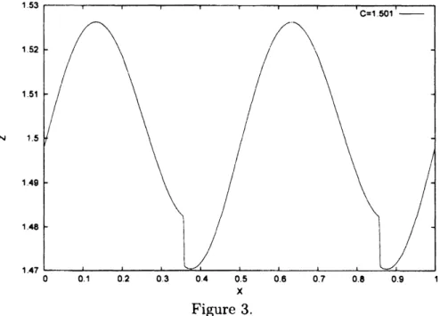
Figure 3.

Figure 3 shows a discontinuous $\mathbb{Z}^{2}$-periodic solution $\overline{u}^{C}$ with _{$t1_{1}e$}

mornentum $C=1.501$

.

We took $N=60000$ as the number of meshes on x-axis in oder to make the shocks

sharpen. The dynamics ofcharacteristic

curves

around thisgraph is visualized in Figure

$\triangleright 1$

Figure 4.

In Figure 4,

we

see

two

characteristic curves

forming

a

curve-like set and in between

three characteristic

curves

forming a pair of islands. The dynamics may have

on

the

Poincar\’e _section

_a

pair _{of elliptic points with elliptic islands and a pair of hyperbolic}

points with the stable/unstable curves. We put Figure 3 and 4 together in Figure 5.

$N$

X

Figure 5.

We

can

say that Figure 5 indicates the situation where the smooth parts of the

discon-tinuous graph

are

pieces of the unstable

curves

arid the

shocks

are

across

the

elliptic

X

Figure 6.

Figure

6

illustrates discontinuous $\mathbb{Z}^{2}$-periodic solutions $\overline{u}^{C}$

with the momentum $C=$

0.7, 0.05, $-0.2$. The dynamics around their graph is “chaotic”. The scattered dots

are

formed by a characteristic

curve

$c(s)$ wandering wide range of the space. The previous

relation between $t1_{1}e$ discontinuous graph and $t$}_$)e$ unstable

curves

is not so clear.

References

[1] V. I. Arnol’d, Proof of

a

theorem of A. N. Kolmogorov

on

the persistence of

quasi-periodic motions under small perturbations of the Hamiltonian, Russ. Math.

Surv.

18 (1963), No. 5, 9-36.

[2]

E.

Fermi,

J.

Pasta,

S.

Ulam,

Los Alamos

report

LA-1940.

(In

E.

Fermi,

Collected

Papers II (1955), Univ. Chicago Press (1965), 977-988.)

[3] H. R. Jauslin, H. O. Kreiss, J. Moser, On the forced Burgers equation with periodic

boundary conditions, Proc. Sympos. Pure Math. 65 (1999), 133-153.

[4] A. I. Khinchin (trans. by G. Gamow), Mathematical foundations of statistical

me-chanics, Dover (1949).

[5] A. N. Kolmogorov, Preservation of conditionally periodic motions for a small change

in Hamilton’s function, Dokl. Akad. Nauk

SSSR

98 (1954), No. 4, 527-530.

[6] J. Moser, E. J. Zehnder, Notes on dynamical systems,

Courant

Lecture Notes in

Mathematics 12 (2005),

[7] T. Nishida, A note

on an

existence of conditionally periodic oscillation in

a

[8] O. A. Oleinik, Discontinuous solutions of nonlinear differential equations, A. M. S.

Transl. (ser. 2) 26 (1957), 95-172.

[9] M. B. Sevryuk, The

classical KAM

theory at the dawn of the twenty-first century

(To V. I. Arnold

on

the occasion of his 65th birthday), Mosc. Math. J. 3 (2003),

no.

3, 1113-1144, 1201-1202.

[10] S. Takeno, Time-periodic solutions for a scalar conservation law, Nonlinear Anal.

45 (2001),

no.

8,

1039-1060.

[11] W. $E$, Aubry-Mather theory and periodic solutions of the

forced

Burgers _equation,