A Threshold Model for Discontinuous Preference
Change and Satiation
著者
Terui Nobuhiko, Hasegawa Shohei, Allenby
Greg M.
journal or
publication title
TMARG Discussion Papers
number
122
year
2015-10
TOHOKU MANAGEMENT
&ACCOUNTING RESEARCH GROUP
Discussion Paper No. 122
A Threshold Model for
Discontinuous Preference Change and Satiation
Nobuhiko Terui
Shohei Hasegawa
Greg M. Allenby
October, 2015
GRADUATE SCHOOL OF ECONOMICS AND MANAGEMENT TOHOKU UNIVERSITY KAWAUCHI, AOBA-KU, SENDAI 980-8576 JAPAN
1
A Threshold Model for
Discontinuous Preference Change and Satiation
by
Nobuhiko Terui
Graduate School of Economics and Management Tohoku University
Sendai, Japan [email protected]
Shohei Hasegawa
Faculty of Business Administration Hosei University
Tokyo, Japan
and
Greg M. Allenby Fisher College of Business
Ohio State University Columbus, Ohio [email protected]
April, 2013 May, 2015 October, 2015
2
A Threshold Model for
Discontinuous Preference Change and Satiation
Abstract
We develop a structural model of horizontal and temporal variety seeking using an dynamic factor model that relates attribute satiation to brand preferences. The factor model employs a threshold specification that triggers preference changes when customer satiation exceeds an admissible level but does not change otherwise. The factor model can be applied to high dimensional switching data often encountered when multiple brands are purchased across multiple time periods. The model is applied to two panel datasets, an experimental field study and a traditional scanner panel dataset, where we find large improvements in model fit that reflect distinct shifts in consumer preferences over time. The model can identify the product attributes responsible for satiation, and can be used to produce a dynamic joint space map that displays brand positions and temporal changes in consumer preferences over time.
Key words and phrases:
3
A Threshold Model for
Discontinuous Preference Change and Satiation
1. Introduction
Consumers purchase a variety of goods in every product category, and invariably switch brands at some point in time because of deals or because they get tired of consuming the same products. Temporary changes in preference have been the subject of a long literature on variety seeking in marketing, with reasons ranging from the presence of multiple needs, persons and contexts, to changes in tastes, constraints and available offerings (see McAlister and Pessemier, 1982). This paper investigates the relationship between satiation and preference as an explanation for why people seek variety. We find that consumer satiation affects preferences in a predictable way up to a point, after which consumer preferences abruptly change and consumers switch to varieties that are distinctly different from those consumed in the past. Our findings have implications for the breadth of products carried by retailers.
Existing models of variety seeking assume that changes in the demand for varieties can be explained by a continuous model structure with predictable changes in preference. Models of horizontal variety seeking (Kim et al. 2003, Bhat 2005), for example, assume that diminishing marginal returns (i.e., satiation) explain why people purchase multiple varieties, where marginal utility is a function of quantity purchased. In these models people are assumed to have stable preferences that diminish in intensity as consumption quantities increase, leading them to tire of consuming large quantities.
Variety seeking behavior is also modeled by including lagged purchase variables in models of discrete choice (Dube, Hitsch and Rossi 2009 , Chintagunta 1998). A positive coefficient value for lagged purchase leads to higher repurchase probabilities for the consumed product while leaving the preference ordering for the remaining varieties unaffected. Models with lagged purchase variables make relatively minor changes to the preference ordering unless multiple lagged variables are
4 included in the model specification.
A problem common to the study of temporal and horizontal variation of brand purchases is with the dimensionality of switching behavior. The study of N brands is associated with N2 different
possible "switches" for two time periods if only one brand is purchased. The dimensionality increases when considering the temporal variation of horizontal variety, where multiple goods are purchased in both time periods. Models of switching behavior are challenged by the large number of possible purchase outcomes, even when the number of brands under study is relatively small.
In this paper we propose a model of preference change that distinguishes multiple forms of variety seeking and examines the temporal relationship between product satiation and brand preference. We find that preference changes are initiated from a latent satiation variable that varies over time, which is related to brand characteristics that also drive baseline preferences. Consumer preferences are stable for a period of time, and then abruptly change when the latent satiation variable exceeds a threshold value. This behavior is consistent with consumers becoming tired of consuming the same set of products and then moving on to a new set. Our threshold model relates product attributes to switching behavior and can identify which product attributes are responsible for the change, and has implications for the breadth of offerings carried by retailers.
We address the issue of dimensionality by employing a dynamic factor model that relates preference and satiation. The factor model allows for continuous variation in product satiation parameters, and the factor loadings point to product attributes responsible for variation in the satiation parameters. The dynamic satiation factor is also used to explain variation in brand preference parameters through a second set of factor loadings. We find that the best fitting model has the preference factors changing only when the dynamic satiation factor exceeds a threshold.
The organization of the paper is as follows. In Section 2 we introduce our model and contrast it to existing models of horizontal and temporal variety seeking. We include a discussion of alternative models examined in our empirical analysis that relax some of the assumptions of our
5
proposed model. Section 3 describes two empirical applications – one using experimental data of corn chip consumption and the other using a scanner panel dataset of yogurt consumption. In both cases we find significant improvement in model fit over existing models. Section 4 contains a discussion of the results for the two datasets, illustrating the insights provided by the models. Concluding remarks are offered in Section 5.
2. Model
Models of discrete behavior, characterized by thresholds and switching regimes, have been found to provide an accurate description of many aspects of consumer behavior. Behavior decision theory (Einhorn and Hogarth, 1981), for example, describes the effects of framing on consumer decision processes that reflect discrete differences in how consumers view consumption opportunities. The most widely known example of this is how consumers react to gains and losses (Thaler, 1985), but more broadly the similarity, attraction and compromise effects regularly documented in models of choice (Roe, Busemeyer and Townsend, 2001) point to discrete and discontinuous effects in the decision process. The behavioral decision theory literature (e.g., Kahneman and Tversky, 1979) indicates that human behavior reflects discrete, not continuous changes as choice alternatives are described, framed and presented to consumers.
The modeling literature in marketing has also found that models with discrete thresholds provide a good description of marketplace behavior. Switching regression models (Terui and Dahana, 2006), models of structural heterogeneity (Kamakura et al. 1996), and Markov switching models (Fruhwirth-Schnatter, 2006) all describe different response processes among and within respondents. Fong and DeSarbo (2007) propose a model of choice in which consumers can enter a passive state of response once they become fatigued. Gilbride and Allenby (2004) propose a choice model with screening component that sets the choice probability to zero if a brand does not enter a person's consideration set. Terui et.al (2011) found that media advertising for mature products
6
affects brand consideration and choice as long an advertising stock variable is above a threshold variable.
We develop our model within the framework of direct utility maximization (Kim et al. 2002, Bhat 2005 and Hasegawa et al. 2012). Consumer h’s utility over j 1, … , m varieties at time t are defined as:
U , z ∑ ln γ x 1 ln z , (1)
where x , … , x is the vector of quantity demanded by consumer h at t , z represents the outside good, and ψ , γ j 1, … , m are parameters restricted as ψ 0 and γ 0. ψ is the baseline value of marginal utility for a product j when x 0, and γ is a satiation parameter that affects the rate at which marginal utility diminishes.
The utility function in (1) is additively separable in the choice alternatives implying that the goods are substitutes and the utility generated by one good is not influenced by the amount of another good purchased. Below we re-parameterize the satiation parameter in terms of product characteristics and other modeling components that are common across the m goods. Thus, while utility is additively separable in terms of the product quantities purchase, changes to product attributes and variables relating to the components can affect multiple goods. An alternative approach assumes that utility is generated by a characteristics (Lancasterian) model as in Chan (2006). However, this approach requires the introduction of interaction terms to overcome the separability restrictions, and assumes that there are not unobserved product characteristics. Our approach instead relies upon the use of a low-dimensional factor model to relate the goods so that the marginal utility of a characteristic (c), i.e., , is not additively separable in the choice alternatives.
A stochastic model is obtained by assuming that the baseline utility parameter has an error, or that ψ exp ψ∗ ε where ψ∗ and ε are unrestricted and independent errors,
7
respectively. Then, the likelihood function is obtained by maximizing (1) subject to the budget
constraint ′ z E , where and , respectively, mean price and quantity vector, and E is the total expenditure. This is accomplished by creating the auxiliary equation as follows:
Q U , z λ ′ z E . (2)
By employing the Kuhn–Tucker conditions of constrained utility maximization, we obtain an expression that relates the observed demand to the error terms as follows:
ε ψ∗ ln γ x 1 ln p
E p′x if x 0 (3)
ε ψ∗ ln γ x 1 ln
′ if x 0. (4)
Then, the likelihood function is composed of a combination of density and probability mass, arising from the interior and corner solutions, respectively. We assume that it follows independently normal distribution ε ~N 0, 1 , as developed in Hasegawa et al. (2012).
Baseline and Preference Dynamics with Switching Structure
We assume that the baseline parameters are well projected into a lower-dimensional space, as is done in a choice map when conducting a market structure analysis (Hauser and Shugan 1983, Elrod 1988, Chintagunta 1994, Wedel and DeSarbo 1996):
∗ ; ∼ N 0, V diag v , … , v . (5)
Each row vector of factor loadings matrix defines the coordinate of brand position and corresponding factor score vector , indicating consumer h’s preference direction at time t. We will refer to as the preference direction vector. We assume that the preference direction will change when consumer satiation level exceeds the admissible level r , but does not change otherwise. Then, the first dynamic factor model is described as follows:
8
f∗ ; ∼ N 0, I if f∗ r
if f∗ r , (6)
where β , β ′ and we set the hierarchical model as β ∼ N β , 1 k 1, 2. The factor ∗ is described below in our model for satiation dynamics. We set r 0 for identification in the empirical application.
Our formulation is consistent with existing models in the marketing and psychology literatures. The dynamic attribute satiation (DAS) model of McAlister (1982) and McAlister and Pessemier (1982) predicts that variety seeking occurs as a respondent's consumption history evolves. Sarigollu (1998) extends the DAS model to include a discrete choice model where preferences are related to an inventory of past attribute accumulation. Our formulation includes the discrete choice model as a special case, and incorporates threshold effects (rh) leading to discrete changes in preference. The
model explains observed choices through the parameters of the choice model (e.g., ∗ ) that vary through time according to a dynamic factor model specified in equations (5) and (6). One possible motivation for our model is the single peak model by Coombs and Avrunin (1977) in which consumers reach an optimal level of an attribute and then, because of their satiation, decide to consume a different attribute on the next purchase occasion. We investigate changing preferences for brands through a dynamic factor model with a loading matrix that, as we see below, helps visualize spatial patterns of competition.
Satiation Dynamics
We relate satiation parameters to brand characteristics using information provided to us by the product manufacturer in a linear mapping, similar to that found in conjoint analysis. They are used as γ∗ c α , and are organized in a matrix form by
∗ , (7) where γ∗ exp γ , c is a vector of characteristics for the j product of dimension p, and
9
is the matrix constituted by a row vector. Thus, product satiation at time t, γ∗ , is assumed to be linearly related to the satiation of the attributes . We further assume that attribute satiation follows a dynamic factor model with a time-invariant factor loading matrix and one-dimensional factor f :
f ; ∼ N 0, Σ diag σ , … , σ (8) f f ν ; ν ∼ N 0,1 . (9) The satiation factor score f is specified a priori in (9) as a random walk, which imposes a smoothness prior on changes in the factor over time. The random walk specification allows for the accumulating effects of past purchases, where parameter values of high likelihood rationalize the observed choices. Equation (9) defines a non-parametric model for temporal dynamics, and it accommodates a trend component locally linear over time in the non-stationary part worth and satiation parameters. This specification has been successfully used in state space modeling (See the literatures in time series analysis, e.g., Harvey (1989), Kitagawa and Gersh (1984), West and Harrison (1997), Terui et al. (2010), and Terui and Ban (2014)).
The factor score moves rather smoothly when the variance of factor score is smaller than the part worth’s variance, as is employed and discussed in Hasegawa et al. (2012). When multiplied by the factor loading matrix , the result is a vector of attribute satiation coefficients that evolve through time with expected value f . Thus, the factor loading matrix can indicate for which of the product attributes consumers experience temporal variation in satiation.
Alternative Models
We compare our model with six alternative models. The first model employs a static preference direction using an ordinary factor model, and is denoted as (Static).
∗ ; ∼ N 0, V diag v , … , v . (10)
10 effects.
The second alternative is a dynamic model that assumes the preference direction vector follows a random walk:
; ∼ N 0, I . (11)
This specification is identical to a non-parametric model of a stochastic trend in time series . Equation (11) has no causal variables or structural parameters, and we refer to this model as a non-parametric dynamic factor model (NDF). This specification was successfully employed in Hasegawa et al. (2012) to capture the locally linear stochastic trend for a non-stationary series.
The third model specifies the preference direction vector as being related to satiation in the previous period:
h1fht 1∗ ; ∼ N 0, I . (12) We call the model represented by (12) as the structured dynamic factor model (SDF). Both the NDF and SDF have a common property that preference changes whenever a consumer purchases a product.
The next set of models has a switching mechanism regarding the timing of preference change. We assume that satiation drives the change when its level exceeds a threshold value, and does not drive the change otherwise. These models have various forms, or types. The first is an SDF model with threshold switching, called a switching non-parametric dynamic model (SNDF):
; ∼ N 0, I if f∗ r
if f∗ r (13)
The second model is our proposed switching structured dynamic factor model (SSDF1) shown in (6). The third model is composed of the two previous models, called a hybrid dynamic factor model (SSDF2):
h1fht 1∗ ; ∼ N 0, I if f∗ r
11
This model provides a flexible specification of the preference vector updating equation, allowing the current preference vector to be influenced by both the satiation variable and the past preference vector. It allows the expected preference vector to the informed by the satiation variable but not entirely dependent on it.
The fourth model includes an autoregressive term ( ) in the model to allow for greater flexibility relative to equation (14). This model is referred to as SSDF3:
h1fht 1∗ h2 ; ∼ N 0, I if f∗ r
if f∗ r (15)
These models provide a comprehensive set for assessing the benefit of the proposed dynamic model for describing preference change. Table A provides a summary of the alternative model specifications:
== Table A ==
3. Empirical Application
We apply the model to two datasets, an experimental dataset of corn chip consumption of undergraduate students at a large U.S. university, and a scanner panel dataset of yogurt consumption.
3.1 Field Experiment Data Data and Variables
Students were recruited for the experiment if they frequently purchased salty snacks for personal consumption. Students were allocated a $2.00 weekly budget and asked to purchase among eight varieties of corn chips. The offerings were priced at $0.33, allowing the students to select up to six packets each week. The regular price of a corn chips packet was $0.99. The students were told that any unused budget allocation would be paid in cash at the end of the experiment. By offering the chips at reduced prices, we hoped to induce higher levels of consumption, which might provide useful information about satiation. Students were instructed to purchase the chips for their own
12
consumption, not for the consumption of others. These data were previously analyzed by Kim et al. (2009) using a subset of product characteristics and a stationary demand model.
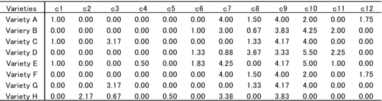
Table 1lists the offerings and associated product characteristics that were provided by the corn chips manufacturer. The chip varieties and characteristics are disguised for proprietary purposes, but reflect summary taste characteristics such as “citrus,” “red pepper,” and “treated corn” that are meaningful to the manufacturer. The experiment was conducted over a seven-week period, resulting in a total of 634 observations for 101 subjects. The data for each purchase occasion is composed of a vector of purchase quantities of each of the eight corn chip varieties, and the quantity of the outside good that was set equal to the unspent budget allocation. Previous analysis of a portion of the characteristics reported in Table 1 indicated that product characteristics could successfully be related to baseline utility in a static model of a choice model.
== Table 1 ==
Summary statistics of the data are reported in Table 2. Very few of the purchase occasions resulted in a corner solution where just one of the varieties were selected. Purchase incidence of the varieties ranged from 168 to 244, indicating that no variety was dominant in the data. The prevalence of interior solutions points to the need for a demand model that can accommodate interior solutions.
== Table 2 ==
Model Comparison
We employ Bayesian MCMC methods to evaluate the joint posterior density for these models. Algorithms for model estimation are provided in the appendix. Models converged relatively quickly and were estimated on the basis of 20,000 iterations of the Markov chain after 10,000 burn-in samples. The interpretation of satiation parameters and the number of factors are robust throughout the models.
Table 3 reports two measures of model plausibility for each model: the log marginal density (ML) and Bayesian deviance information criterion (DIC). The DIC is a measure of model
13
comparison that explicitly penalizes a model for its number of parameters (Spiegelhalter et al., 2002). We use the DIC instead of calculating model performance on a holdout set of data because our student panel experienced a fair amount of attrition toward the end of the study, particularly in the sixth and seventh weeks. The loss of data toward the end of the panel makes it difficult to compare the out-of-sample predictions, particularly with dynamic models. The results indicate that the models differ greatly in their fit to the data.
== Table 3 ==
First, we find that incorporating dynamics into the baseline parameters ψ leads to a dramatic improvement in model fit in terms of criteria by observing dramatic improvement between the static and dynamic models. The static model fit shows DIC = 11067.6, and log ML = −5088.8. On the other hand, the dynamic models have approximately 80% lesser DIC and 60% greater log ML values. The fit results indicate that consumer variety seeking behavior is episodic, with regime changes in tastes as predicted by our model and explained by increased levels of satiation. Second, a comparison among the dynamic models shows that the switching models dominate the steady changing models in both criteria. That is, preferences change discretely in relation to the level of satiation in the previous period.
The best-fitting model is our proposed model (SSDF1). In this model, preference changes are represented by discrete switches related to previous levels of satiation. The next best model is the switching structured dynamic factor autoregressive model (SSDF3), indicating that a parametric specification is better than a non-parametric local trend specification (SNDF and SSDF2).
Parameter Estimates
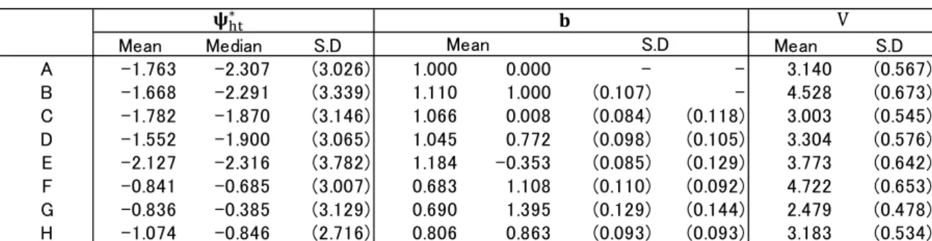
Table 4 summarizes the posterior distributions of parameters for the model SSDF1, the best-fitting model.
14
The top portion of the table, Table 4(a), reports estimates of parameters in the dynamic factor model for the baseline parameters across households and over time. Since the posterior distributions of some of these quantities are skewed, we also report the posterior median when needed. We observe that the estimated baselines ∗ for products are almost proportional to their shares in purchase records. The factor loading matrix , as well as the variance matrix V, are almost significantly estimated.
The middle portion of the table, Table 4(b), reports the posterior mean and median for coefficient parameters in the switching equation. The satiation level f explains the direction of preference in the first dimension as E β 1.323 standard deviation S. D. ∶ 0.885 . On the other hand, it does not affect the second dimension as E β 0.112(S.D.:0.854).
The bottom portion of the table, Table 4(c), reports estimates of parameters in the dynamic factor model for brand satiation, i.e., product attribute part-worth on satiation, factor loadings, and variances. The estimates for and have opposite signs, implying that f represents an excitement (anti-satiation) factor score, the same as that shown in Hasegawa et al. (2012). The estimates of part worth mean the importance weights of product characteristics c1-c12 on the
satiation. The characteristics (c4, c5, c10, c12) have positive large numbers of estimates, indicating that these characteristics contribute to brand satiation. In contract, (c1, c8, c11) with negative large values are characteristics that reduce consumer satiation. Finally, (c2, c3, c6, c7, c9) have almost zero impact on satiation.
== Figure 1 ==
Figure 1 depicts a histogram of individual consumer propensity score k to change their preference. The score is defined by
k k T (20) where k ∑ k ⁄ is the posterior probability of consumer h’s changing preference at period R
15
t across R iterations of MCMC, and k is the indicator taking binary according to the switching mechanism
k 1 if f
∗ 0
0 if f∗ 0 (21) The figure shows that many consumers change their preference, as E k = 0.791 and the share of consumers with k 0.8 is 71.3%. Thus, while about 20% of the consumers exhibit stable preferences, the remainder exhibit changes in baseline preferences over the course of their purchase history.
== Figure 2 ==
Figure 2 shows histograms of estimated coefficients on the switching equation. The left and right figures are the estimates of β for the first dimension of the preference direction and those of β for the second dimension, respectively. The heterogeneous distribution across consumers is relatively stable, although slightly skewed to the right for β . E β 1.323 and E β 0.112. Considering the relation gg ββ f∗ ωω , this means that the satiation level affects the first dimension more than the second dimension.
3.2 Market Data- Scanner Panel Data Data and Variables
The second dataset is the scanner panel data of yogurt category, which was used in Kim et al.(2002). It contains five popular flavors of Dannon yogurt - blueberry, mixed berry, pin a colada, plain, and strawberry- in eight ounce size, and their purchase records are restricted to only those households with more than one purchase occasion for at least one of our five varieties. This yields a data set with 332 households and 2,380 purchase observations. However, we extracted 127 households with more than five purchase records in order to keep holdout samples for evaluating RMSE of forecasts. The data is summarized in Table 5.
16
We note that total counts and proportions in the bottom row are calculated based on the number of brand purchases (not purchase incidences) in conformity with experimental data in section 3.1. We observe that this dataset has 41% interior solutions among 2,109 brand purchases, and it suggests weaker satiation on the category than the case of experimental data. We also denote that five flavors have an identical price which is changing over time.
== Table 5 ==
Model Estimation
This dataset does not contain the precise information on consumer’s budget, i.e., the amount of outside goods, and this situation leaves the equilibrium level of λ undetermined. In this case, we constitute the likelihood based on relative likelihood by taking difference of respective brand’s conditions from that of a specified brand, as is done by Kim et al. (2002).
That is, let D ψ∗ ln γ x 1 ln p , then the Kuhn-Tucker conditions (3) and (4) lead to
ε D ln λ if x 0 ε D ln λ if x 0
and we take difference from a purchased brand k at t for h in order to get rid of the term ln λ from these equality and inequality equations respectively, then we have
e V if x 0 (22) e V if x 0 (23) In the above, we define e ε ε and V D D , where k means the index for a purchased brand at t for h.
Then if we assume that ε follows a standard normal distribution, the derived error terms e ′s follow the reduced dimensional multivariate normal distribution with e e , e , … , e ~ 0, Σ , where the diagonal elements of variance covariance matrix are V e 2, and offdiagonal elements are Cov e , e 1 . In this case, the
17
probability mass for non-purchase occasions after arranging terms for non-purchase brands into latter positions ordering by 1, … , 1,
Pr x 0, 1, … , 1
⋯ e , e , … , e de de … de (24)
can be evaluated via GHK simulator.
The dataset does not contain product characteristic information, and we directly apply dynamic factor model to satiation parameters ∗ . That is, we define the product characteristics matrix in (7) as the identity matrix in this analysis.
== Table 6 ==
Model Comparison
Table 6 shows the results of model comparison. In addition to log ML as in-sample criterion, we directly evaluated the RMSE of forecasts as out of sample criteria because we could keep holdout samples. The same conclusions are derived by these criteria as those obtained in experimental data. That is, incorporating dynamics improves model fit significantly, and the dynamic structured models with switching structure perform substantially better. Both criteria suggested SSDF1 as the best model.
== Table 6 ==
Parameter Estimates
The parameter estimates are shown in Table 7. The panel (a) shows that the estimated baseline parameters are significant in the sense of posterior t ratio from grand means and S.D.’s, and they are proportional to purchase shares which justify our estimates. The factor loadings as well as their variances are also significantly estimated. We note that the baseline parameter for brand E is set as 0 for identification. The panel (b) denotes the coefficient estimates on the previous satiation level. We observe that the previous level of satiation positively affects first dimension of preference vector
18
and it has a lesser influence on the second dimension in opposite direction. == Table 7 ==
== Figure 3 == == Figure 4 ==
Figure 3 illustrates the heterogeneity distribution of individual propensity score of preference change. The heterogeneity distribution is similar to that found for the experimental data. Figure 4 shows the distribution of heterogeneity on the coefficients of switching equations.
4. Discussion
In this section, we investigate model implications using the experimental data. Results from the scanner panel dataset are similar and are available upon request. First, we investigate the implication of our model of preference dynamics by comparing the compensating values (CV) implied by the dynamic factor model to those from the traditional static model. The results indicate that varieties are more highly valued with the proposed dynamic model, implying that consumer highly value wide assortment. We also examine the dynamics of preference change by considering three panelists with three preference patterns that exhibit frequent changes over time, moderately frequent change, and non-changing preferences, and consider how estimates for individual consumers are related to observed purchase behavior and switching structure. The dynamic joint space maps are depicted.
4.1 Compensating Values
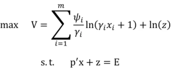
Following Kim et al.(2002), we compute the compensating value (CV) of the offerings that allows us to assess the value of an assortment. The CV is computed by first computing the utility of the observed choices from our utility model:
19
max V ln 1 ln
s. t. p x z E
(24)
The posterior mean of parameters ψ, γ and the observed values of p, E are inserted in (24) to obtain x and V. We then delete brand i and search for the value of CV so that V and V are equal:
V p , E V p , (25)
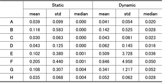
Table 8 provides a comparison of the posterior means of CV for the static and dynamic models, where the latter model takes grand mean over time, and table 9 expresses CV as a share of budget
∑ .
Reported in Tables 8 and 9 is the mean and standard deviation of heterogeneity of the compensating value statistics. We also report the median of the distribution because of the distribution of values is highly skewed. The results imply that the static model severely underestimates CV for every brand and, as a result, undervalues product assortment. Our model of discontinuous preference change leads to larger estimates of the value due to the occasions for which there is strong preference. Compensating values calculated for the static model are lower because preference estimates are averaged over the entire purchase history of the consumer, resulting in varieties that appear to be closer substitutes. Our dynamic model supports the existence of wide assortments, whereas the static model does not.
== Table 8 == == Table 9 ==
4.2 Preference Dynamics
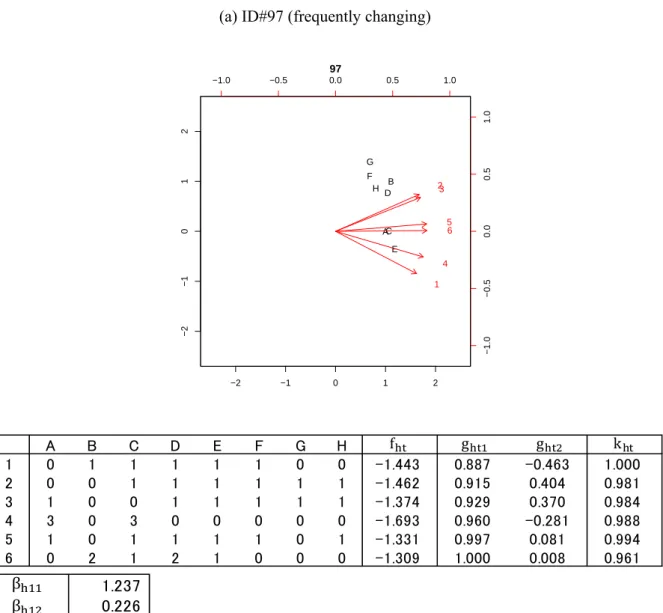
20
#97 in the experimental dataset. The purchase records indicate multiple purchases with a broad range, a satiation score (minus f value) that remains at a high level, and then the switching mechanism works such that the coordinates in the attributed space move all the time. This consumer can be characterized as a variety seeker. The satiation (excitement) level affects both coordinates positively, and this impact is much greater for the first dimension.
== Figure 5 ==
Figure 5(b) provides the map and tables for panelist #35, showing moderately frequent change. Preference changes up to the third time purchase, but does not change anymore after this period. We note that the preference direction is not heading to any product during the first period, and four varieties of corn chips of a single quantity were purchased at this time. This could imply that she was unfamiliar with this product category and getting excited as she purchased them. The satiation (excitement) level negatively and positively affects the first and the second coordinates to change, respectively.
Figure 5(c) provides the map and tables for panelist #15, showing no preference changes. The record for purchasing D is consistent with the preference direction. The satiation (excitement) level negatively and positively affects the first and second coordinates to change, respectively, and it is much greater for the first coordinate. Figures 5(a)-(c) demonstrate the flexibility of the proposed dynamic model for studying preferences.
5. Concluding Remarks
In this paper we develop a parsimonious model of dynamic variety seeking that relates preference changes to brand satiation. Two dynamic factor models are developed for baseline and satiation parameters in a direct utility model of horizontal variety that are integrated so that preference can change abruptly when the satiation factor score exceeds a threshold level. We find strong empirical support for our model in two datasets, and show how the model can be used to identify
21
product characteristics responsible for satiation. Our model is motivated by theories of adoption and change similar to McAlister (1982) and McAlister and Pessemier (1982), who proposed a framework for relating satiation to preference. The presence of different operating regimes also has a long history in the marketing and psychology literatures (e.g., Coombs and Avrunin, 1977).
We compare our model to alternative specifications, including a static model implying that preference does not change at all, a dynamic model without a switching structure on preference change, and dynamic models with switching structures. The models in the last category are composed of non-parametric local linear trend, parametric regression, and their hybrid models. The measures of model fit, log of ML and DIC support the model with a switching structure and parametric regression. This means that preference will change occasionally after a consumer is satiated enough, and that it stays the same until the critical level.
The empirical applications demonstrate that abrupt preference changes are common across consumers, with 70% or more changing their preferences over the course of their purchase history. The results indicate that the standard modeling assumption of static preferences in problematic, particularly in light of the large increase in model fit for our proposed dynamic models. We find that consumers with wider varieties of purchases tend to change their preferences more often – that is, through periodic shifts in preference as described by the model. This finding is consistent with consumers having well defined tastes that vary through time, as opposed to broad tastes for which many brands will suffice. Our results are consistent with emerging evidence of binge behavior, or "clumpliness" in consumer demand that is not consistent with the notion of stable preferences (Zhang, Bradlow and Small, 2015).
Future research is needed to understand the context of purchase and consumption. Our results indicate that the unit of analysis for heterogeneity is not the respondent, but instead the respondent at a specific purchase occasion who is influenced by their past decisions and other factors. Additional work is needed to identify and integrate these factors and past events into models of consumer
22
decision making that allow marketers to anticipate shifts in preference. We believe that the temporal study of satiation, and other triggers of preference change, is a fruitful area for future research.
Appendix – Identification Condition and MCMC Algorithm
We explain the identification condition for the dynamic factor model, and summarize the prior and conditional posterior distribution used for our proposed one-factor model below.
1. Identification Condition on and Priors for Factor Models
For a two-factor model applied to baseline parameters, we restrict the loadings to achieve statistical identification: 1 a 01 a ⋮ a a ⋮ a (A.1)
This restriction due to the factor model being applied to parameters of a latent utility is stronger than Geweke and Zhou’s (1996) condition for the conventional factor model.
We then define prior distribution of factor model as:
σ ∼ IG n /2, s /2 (A.2) a ∼ N a , A ; a , a ′∼ N , for 3 k p, (A.3) as suggested in Lee (2007). The first column of (A.1) is set on factor loadings for a one-factor model applied to satiation parameter. The following same prior distributions are employed
v ∼ IG n /2, s /2 (A.4) b ∼ N b , B for 2 k p, (A.5)
2. Prior Distributions on Hyper Parameters
Prior Setting a ∼ N a , A a 0, A 100 ∼ N , , 100 ∼ N , , β0 10 v ∼ IG n ⁄ , s2 ⁄ 2 n 2, s 2 σ ∼ IG nσ ⁄ , s2 σ ⁄ 2 nσ 2, sσ 2
23 3. Conditional Posterior Distributions for MCMC
As for the experimental data, we run 20,000 MCMC iterations for all models, and we used last 10,000 iterations to calculate posterior distribution of model parameters. The analysis for scanner panel data needs 40,000 MCMC iterations for all models, and we used last 20,000 iterations to calculate posterior distribution of model parameters.
(1) ∗ | , , , ,
p ∗ | , , , ,
∝ det| | ⁄ exp ∗ ′ ∗ ⁄2
L ∗
(A.6)
The term L ∗ is the likelihood function for consumer h 1, … , H at purchase time t 1, … , T , where the likelihood function is composed of a combination of density and mass, arising from the interior and corner solutions, respectively, and is defined for experimental data as
, … , | | ⋯ , … , ⋯
where the probability mass is evaluated in computation by calling function of univariate normal distribution function. Fore scanner data, the likelihood is defined similarly as (24), where multiple integrals are evaluated by GHK simulator.
Setting r 1, … , R to MCMC iterations, we use Metropolis–Hastings with a random walk algorithm, each h 1, … , H and t 1, … , T .
∗ ∗
ψ; ψ ∼ N 0, (A.7)
The tuning parameter k was chosen as 0.5 for experimental data, and 0.8 for scanner panel data. The acceptance probability is
min p ∗ , , , , p ∗ , , , , , 1 (A.8) (2) | , ∗ , , f , p | , ∗ , , f , ∝ det| | ⁄ exp f ′ f ⁄2 L (A.9)
As for ∗ , we use Metropolis–Hastings with a random walk algorithm, each h 1, … , H and t 1, … , T .
α; α∼ N 0, ′ (A.10)
The tuning parameter k’ was chosen as 0.01 for experimental data, and 0.6 for scanner panel data. The acceptance probability is
24
min p ,
∗ , , ,
p , ∗ , , , , 1 (A.11)
(3) | , f ,
Under the assumption of uncorrelated a ’s, we define f , f , ⋯ , f ′: T 1 matrix, and then make downward stacking over h, ′, ′, ⋯ ; ′ ′ : ∏ T 1 matrix. Similarly, we define α , α , … , α ′: T 1, and ′ , ′ , ⋯ , ′ ′ : ∏ T 1. Then, we have the regression equation with coefficient parameter vector and explanatory matrix .
a ∼ N a , A , (A.12)
where
A A σ ′ , a A A a σ ′
The identification condition is considered when k 1 .
(4) | ∗ , ,
In the same way as , we define , , ⋯ , ′: T 2 matrix,
′, ′, ⋯ ; ′ ′ : ∏ T 2 matrix and ∗ ψ∗ , ψ∗ , … , ψ∗ ′: T 1,
∗ ∗ ′, ∗ ′, ⋯ , ∗ ′ ′ : ∏ T 1.
∼ N , , (A.13)
where
v ′ , a v ′ ∗
The identification condition is considered when j 2 .
(5) f , | , ∗ , ,
We reformulate measurement equation (Equations (8) and (13)) and system equation (Equations (9) and (14)).
Measurement equation:
∗ 0 0 f ; ∼ N 0, 0 0 (A.14)
25 f 1 0 K 1 K f ν ; ν ∼ N 0, 10 K0 , (A.15) where β , β ′ and K 1, if f∗ r K 0, if f∗ r , (A.16)
where we define f∗ f by interpreting the factor of anti-satiation for f . We use Carter and Kohn (1994) for a time-varying coefficient in state space model expressed as Equation (A.14) and Equation (A.15)
(6) SSDF1: β , β ′|f , ,
β ∼ N β , ∗′ ∗ 1 k 1,2 (A.17)
where
β ∗′ ∗ 1 ∗′ β
and ∗ . and are the data matrix and vector respectively collected in case of regime f∗ r or K 1 . If ∅ (K 0 at all t), posterior is β ∼ N β , 1 by the homogeneity.
(7) SSDF1: β , β ′|
β ∼ N β , H νβ k 1,2 (A.18)
where β H νβ ∑ β νβ β .
(8) SSFD3: β , β , β , β |f , , , , , | ,
, , and are sampled by MCMC procedure of general hierarchical Bayes regression model similarly as equation (A.17) and (A.18).
∼ N , (A.19)
We use the data and , which are collected in case of regime f∗ 0 or K 1 . If ∅ (K 0 at all t), the posterior density is defined by ∼ N , .
26
References
[1] Bhat, C. R. (2005), “A Multiple Discrete-Continuous Extreme Value Model: Formulation and Application to Discretionary Time-Use Decisions,” Transportation Research, 39 (8) 679-707. [2] Carter, C. K. and Kohn, R. C. (1994), “On Gibbs sampling for state space models,” Biometrika,
81, 541-553.
[3] Chan, T.Y. (2006) "Estimating a continuous hedonic-choice model with an application to demand for soft drinks," RAND Journal of Economics, 37, 2, 466-482.
[4] Chintagunta, P. (1994), “Heterogeneous Logit Model Implications for Brand Positioning,”
Journal of Marketing Research, 32, 304-311.
[5] Chintagunta, P. (1998), “Inertia and Variety Seeking in a Model of Brand-Purchase Timing,”
Marketing Science, 17(3), 253-270.
[6] Coombs, C.H. and G.S. Avrunin (1977), “Single-peaked functions and the theory of preference,”
Psychological Review, 84(2), 216-230
[7] Dubé, J.P., J.H. Günter and P. E. Rossi (2010), “State dependence and alternative explanations for consumer inertia,” The RAND Journal of Economics, Vol. 41(3), 417-445.
[8] Elrod, T. (1988), “Choice Map: Inferring a Product Market Map from Panel Data,” Marketing
Science, 7, 21-40.
[9] Einhorn, H.J. and R. M. Hogarth (1981), “Behavioral Decision Theory: Processes of Judgment and Choice,” Journal of Accounting Research, 19(1), 1-31
[10] Fong, D.K.H. and W.S. DeSarbo (2007), “A Bayesian methodology for simultaneously detecting and estimating regime change points and variable selection in multiple regression models for marketing research,” Quantitative Marketing and Economics, 5, 427-453.
[11] Frühwirth-Schnatter, S. (2006), Finite Mixture and Markov Switching Models, Springer, New York.
[12] Geweke, J. and G. Zhou (1996), “Measuring the Pricing Error of the Arbitrage Pricing Theory,”
The Review of Financial Studies, 9, 557-587.
[13] Gilbride, T. and G. Allenby (2004), “A Choice Model with Conjunctive, Disjunctive, and Compensatory Screening Rules,” Marketing Science, 23 (3), 391-406.
[14] Hasegawa, S., N. Terui and G. Allenby (2012), “Dynamic Brand Satiation,” Journal of
Marketing Research, vol. XLIX, 842-853.
[15] Hauser, J. R. and S. M. Shugan (1983), “Defensive Marketing Strategies,” Marketing Science, 2 (4), 319-360.
[16] Harvey, A. (1989), Forecasting Structural Time Series Models and the Kalman Filter, Cambridge University Press, London.
[17] Kahneman, D. and A. Tversky (1979), “Prospect theory: an analysis of decision under risk,”
Econometrica, 47, 263-291.
27
in Consumer Choice,” Marketing Science, 15 (2), 152-172.
[19] Kim, J., G. Allenby and P. Rossi (2002), “Modeling Consumer Demand for Variety,” Marketing
Science, 21, 229-250.
[20] Kim, J., G. Allenby and P. Rossi (2009), “Product attribute and models of multiple discreteness,”
Journal of Econometrics, 138, 208-230.
[21] Kitagawa, G. and J. Gersh (1984), “A smoothness priors-state space modeling of time series with trends and seasonalities,” Journal of the American Statistical Association, vol.79, 378–389. [22] McAlister, L. and E. Pessemier (1982), Variety Seeking Behavior: An Interdisciplinary Review,
Journal of Consumer Research, 9, 311-322.
[23] McAlister, L. (1982), “A Dynamic Attribute Satiation Model of Variety-Seeking Behavior,”
Journal of Consumer Research, 9, 141-150.
[24] Roe, R. M., J.R. Busemeyer, J.T. Townsend (2001), “Multialternative decision field theory: A dynamic connectionist model of decision making,“ Psychological Review, 108(2), 370-392. [25] Sarigollu, E. and D.C. Schmittlein (1998), “The effect of variety seeking behaviour on optimal
product positioning,” Applied Stochastic Models and Data Analysis, 12(1), 27–44.
[26] Spiegelhalter, D. J., N. Best, B. P. Carlin, and A. van der Linde (2002). “Bayesian measures of model complexity and fit,” Journal of the Royal Statistical Society, Series B, 64 (4), 583-616. [27] Terui, N. and W. D. Dahana (2006), “Estimating Heterogeneous Price Thresholds,” Marketing
Science, 25 (4), 384-391.
[28] Terui, N., M. Ban and T. Maki (2010), “Finding Market Structure by Sales Count Dynamics— Multivariate Structural Time Series Models with Hierarchical Structure for Count Data—,”
Annals of the Institute of Statistical Mathematics, 62, 92-107.
[29] Terui, N., M. Ban and G. Allenby (2011), “The Effect of Media Advertising on Brand Consideration and Choice,” Marketing Science, 30 (1), 74-91.
[30] Terui, N. and M. Ban (2014), “Multivariate Structural Time Series Models with Hierarchical Structure for Over-dispersed Discrete Outcome,” Journal of Forecasting, 33, 376-390. [31] Thaler, R. (1985), “Mental Accounting and Consumer Choice,” Marketing Science, 4(3),
199-214.
[32] Wedel, M. and W.S. Desarbo (1996), “An Exponential Family Multidimensional Scaling Mixture Methodology,” Journal of Business and Economics Statistics, 14(4), 447-459
[33] West, M and J. Harrison (1997), Bayesian Forecasting and Dynamic Models(2nd ed.), Springer,
New York.
[34] Yang, S., G. Allenby and G. Fennel (2002), “Modeling Variation in Brand Preference: The Roles of Objective Environment and Motivating Conditions,” Marketing Science, 21 (1), 14-31. [35] Zhang Y, E.T. Bradlow and D.S.Small (2015), “Predicting customer value using clumpiness:
28
Table A : Summary of Alternative Models1
Model Dynamic Switching Equation Specification
Static No No (10) NDF Yes No (11)
SDF Yes No (12) f∗
SNDF Yes Yes (13) if f∗ r
SSDF1 Yes Yes (6) f∗ if f∗ r
SSDF2 Yes Yes (14) f∗ if f∗ r
SSDF3 Yes Yes (15) f∗ if f∗ r
29
Table 1 Product Varieties and Characteristics
Table 2 Purchase Summary-Experimental Data
Kim et al. (2007)
Table 3 Model Comparison-Experimental Data
Varieties c1 c2 c3 c4 c5 c6 c7 c8 c9 c10 c11 c12 Variety A 1.00 0.00 0.00 0.00 0.00 0.00 4.00 1.50 4.00 2.00 0.00 1.75 Variery B 0.00 0.00 0.00 0.00 0.00 1.00 3.00 0.67 3.83 4.25 2.00 0.00 Variety C 1.00 0.00 3.17 0.00 0.00 0.00 0.00 1.33 4.17 4.00 0.00 0.00 Variety D 0.00 0.00 0.00 0.00 0.00 1.33 0.88 3.67 3.33 5.50 2.25 0.00 Variety E 1.00 0.00 0.00 0.50 0.00 1.83 4.25 0.00 4.17 5.00 1.00 0.00 Variety F 0.00 0.00 0.00 0.00 0.00 0.00 4.00 1.50 4.00 2.00 0.00 1.75 Variety G 0.00 0.00 3.17 0.00 0.00 0.00 0.00 1.33 4.17 4.00 0.00 0.00 Variety H 0.00 2.17 0.67 0.00 0.50 0.00 3.38 0.00 3.83 0.00 0.00 0.00 Varieties Purchase incidence Total purchase quantity Corner solution Interior solution Variety A 168 224 - 168 (1.00) Variery B 177 262 4 (.02) 173 (0.98) Variety C 188 231 - 188 (1.00) Variety D 180 235 - 180 (1.00) Variety E 190 295 2 (.01) 188 (0.99) Variety F 244 446 6 (.02) 238 (0.98) Variety G 235 338 - 235 (1.00) Variety H 218 277 - 218 (1.00) Total 1600 2308 12 (0.01) 1588 (0.99) ML DIC Static -5088.8 11067.6 NDF(Nonparametric) -3124.5 8649.0 SDF(Structured) -3171.8 8756.7 SNDF -2829.4 8435.0 SSDF1 -2754.1 8170.0 SSDF2 -2829.5 8425.9 SSDF3 -2758.1 8283.1 Steady Dynamic Switching Model S
30
Table 4 Parameter Estimate-Experimental Data
(a) Baseline Parameters
These numbers show the grand mean and median of panelist’s estimates over time across panel members. S.D. refers to the standard deviation of heterogeneity for ∗ . Numbers for b and V show the posterior mean and
the posterior standard deviation in parentheses.
(b) Switching Equation: Baseline Parameters
These numbers show the grand mean of panelist’s estimates across panel members.
(c) Satiation Parameters: Characteristic Level
These numbers show the grand mean and median of panelist’s estimates over time across panel members. S.D. refers to the standard deviation of heterogeneity for . Number for and Σ show the posterior mean and the posterior standard deviation in parentheses.
Mean Median S.D Mean S.D
A -1.763 -2.307 (3.026) 1.000 0.000 - - 3.140 (0.567) B -1.668 -2.291 (3.339) 1.110 1.000 (0.107) - 4.528 (0.673) C -1.782 -1.870 (3.146) 1.066 0.008 (0.084) (0.118) 3.003 (0.545) D -1.552 -1.900 (3.065) 1.045 0.772 (0.098) (0.105) 3.304 (0.576) E -2.127 -2.316 (3.782) 1.184 -0.353 (0.085) (0.129) 3.773 (0.642) F -0.841 -0.685 (3.007) 0.683 1.108 (0.110) (0.092) 4.722 (0.653) G -0.836 -0.385 (3.129) 0.690 1.395 (0.129) (0.144) 2.479 (0.478) H -1.074 -0.846 (2.716) 0.806 0.863 (0.093) (0.093) 3.183 (0.534) Mean S.D ∗ V
Mean Median S.D Mean S.D
-1.323 -1.428 (0.885) -1.322 (0.186)
0.112 0.162 (0.854) 0.110 (0.189)
β β
Mean Median S.D Mean S.D Mean S.D
c1 -1.230 -1.396 (1.455) 1.000 - 0.187 (0.058) c2 0.007 0.006 (0.033) -0.003 (0.029) 0.105 (0.026) c3 0.081 0.094 (0.096) -0.064 (0.043) 0.063 (0.012) c4 0.547 0.603 (0.658) -0.441 (0.049) 0.461 (0.107) c5 0.421 0.469 (0.498) -0.336 (0.042) 0.322 (0.056) c6 0.052 0.054 (0.076) -0.042 (0.035) 0.136 (0.024) c7 0.012 0.016 (0.035) -0.010 (0.026) 0.040 (0.006) c8 -0.224 -0.246 (0.262) 0.180 (0.033) 0.069 (0.010) c9 -0.033 -0.033 (0.056) 0.029 (0.020) 0.034 (0.004) c10 0.220 0.253 (0.253) -0.174 (0.037) 0.034 (0.004) c11 -0.129 -0.143 (0.151) 0.102 (0.037) 0.094 (0.019) c12 0.283 0.325 (0.332) -0.226 (0.053) 0.120 (0.028) Σ
31
Table 5 Purchase Summary-Scanner Panel Data
A: Strawberry; B: Blueberry; C: Piña Colada; D: Plain; E: Mixed berry
Table 6 Model Comparison -Scanner Panel Data Varieties Purchase incidence Total purchase quantity A 712 1138 403 (0.57) 309 (0.43) B 366 583 205 (0.56) 161 (0.44) C 392 612 186 (0.47) 206 (0.53) D 226 323 209 (0.92) 17 (0.08) E 413 708 240 (0.58) 173 (0.42) Total 2109 3364 1243 (0.59) 866 (0.41)
Corner solution Interior solution
ML RMSE Static -2668.32 101.94 Steady NDF -1838.09 96.92 SNDF -1697.95 96.85 SSDF1 -1626.99 90.11 SSDF2 -1748.68 102.68 SSDF3 -1759.50 107.59 Model Dynamic Switching
32
Table 7 Parameter Estimate-Scanner Panel Data (a) Baseline Parameters
These numbers show the grand mean and median of panelist’s estimates over time across panel members. S.D. refers to the standard deviation of heterogeneity for ∗ . S.D. refers to the standard deviation of heterogeneity
for ∗ . Numbers for b and V show the posterior mean and the posterior standard deviation in parentheses.
(b) Switching Equation
(c) Satiation Parameter
These numbers show the grand mean and median of panelist’s estimates over time across panel members. S.D. refers to the standard deviation of heterogeneity for ∗. Numbers for and Σ show the posterior mean and
the posterior standard deviation in parentheses.
Mean Median S.D Mean S.D
A 4.235 3.430 (4.884) 1.000 - - - 2.188 (0.429) B 4.334 3.493 (8.067) 1.887 1.000 (0.102) - 3.675 (0.867) C 7.044 5.640 (7.649) 1.003 -0.761 (0.078) (0.113) 2.234 (0.507) D -16.438 -13.807 (17.718) -2.759 1.308 (0.251) (0.234) 14.296 (3.805) E - - - -Mean S.D ∗ V
Mean Median S.D Mean S.D
1.214 1.380 (0.979) 1.213 (0.120)
-0.876 -0.845 (0.887) -0.875 (0.205) β
β
Mean Median S.D Mean S.D Mean S.D
A -3.665 -3.274 (2.923) 1.000 - 1.638 (0.356) B -9.017 -7.883 (7.212) 2.466 (0.121) 1.640 (0.405) C -8.931 -7.789 (7.173) 2.446 (0.190) 1.665 (0.428) D -1.649 -1.435 (1.350) 0.453 (0.221) 2.695 (0.885) E -0.362 -0.363 (0.400) 0.097 (0.063) 2.256 (0.610) ∗ Σ
33
Table 8 Compensating Value (CV)
Static Dynamic
mean std median mean std median
A 0.077 0.198 0.000 0.478 0.627 0.243 B 0.232 1.166 0.000 1.560 6.023 0.328 C 0.060 0.126 0.000 0.499 0.686 0.249 D 0.086 0.251 0.000 0.723 1.723 0.190 E 0.204 0.761 0.001 6.158 44.794 0.353 F 0.410 0.880 0.001 9.132 49.874 0.650 G 0.217 0.613 0.007 4.089 14.403 0.534 H 0.071 0.136 0.007 0.635 0.818 0.333
Table 9 Percent Compensating Value (PCV) as a Function of Expenditure
Static Dynamic
mean std median mean std median
A 0.039 0.099 0.000 0.041 0.054 0.020 B 0.116 0.583 0.000 0.142 0.525 0.028 C 0.030 0.063 0.000 0.043 0.061 0.023 D 0.043 0.125 0.000 0.062 0.145 0.016 E 0.102 0.380 0.001 0.509 3.728 0.036 F 0.205 0.440 0.001 0.846 4.958 0.050 G 0.108 0.307 0.004 0.341 1.217 0.052 H 0.035 0.068 0.004 0.052 0.062 0.028
34
Figure 1 Preference Change -Experimental Data-
Figure 2 Parameter Estimates in Switching Equation -Experimental Data - Frequency 0.0 0.2 0.4 0.6 0.8 1.0 0 1 02 03 04 05 06 0 1 Frequency −3 −2 −1 0 1 0 5 10 15 20 25 30 2 Frequency −2 −1 0 1 2 0 5 10 15 20 25 30
35
Figure 3 Preference Change - Scanner Panel Data -
0.2 0.4 0.6 0.8 1.0 0 2 04 06 08 0
Figure 4 Parameter Estimates in Switching Equation -Scanner Panel Data-
β β −1 0 1 2 3 4 0 5 10 15 20 25 30 −3 −2 −1 0 1 0 1 02 03 04 0
36
Figure 5 Preference Dynamics- Experimental Data
(a) ID#97 (frequently changing)
−2 −1 0 1 2 −2 −1 0 1 2 97 A B C D E F G H −1.0 −0.5 0.0 0.5 1.0 −1.0 −0.5 0.0 0.5 1.0 1 23 4 5 6 A B C D E F G H 1 0 1 1 1 1 1 0 0 -1.443 0.887 -0.463 1.000 2 0 0 1 1 1 1 1 1 -1.462 0.915 0.404 0.981 3 1 0 0 1 1 1 1 1 -1.374 0.929 0.370 0.984 4 3 0 3 0 0 0 0 0 -1.693 0.960 -0.281 0.988 5 1 0 1 1 1 1 0 1 -1.331 0.997 0.081 0.994 6 0 2 1 2 1 0 0 0 -1.309 1.000 0.008 0.961 f g g k 1.237 0.226 β β
37
(b) ID#35 (occasionaly changing)
−2 −1 0 1 2 −2 −1 0 1 2 35 A B C D E F G H −2 −1 0 1 2 −2 −1 0 1 2 1 2 3 A B C D E F G H 1 0 1 1 1 1 0 0 0 -0.485 -0.162 -0.987 1.000 2 0 0 0 2 3 0 1 0 -0.421 0.977 0.212 0.561 3 0 1 0 0 2 0 2 1 -0.068 0.876 0.483 0.506 4 0 2 1 2 0 0 0 1 0.413 0.933 0.359 0.462 5 1 0 2 2 0 0 0 1 1.066 0.992 0.130 0.433 6 0 0 0 2 0 2 0 2 1.583 0.917 0.400 0.297 f g g k -0.462 0.258 β β
38
(c) ID#15 (never changing)
−2 −1 0 1 2 −2 −1 0 1 2 15 A B C D E F G H −2 −1 0 1 2 −2 −1 0 1 2 1 A B C D E F G H 1 0 1 1 1 1 0 2 0 0.865 0.967 0.254 1.000 2 0 1 0 1 1 0 3 0 0.743 0.942 0.335 0.156 3 0 0 0 3 0 0 3 0 0.548 0.840 0.542 0.198 4 0 0 0 3 0 0 3 0 0.810 0.768 0.640 0.204 5 0 2 0 4 0 0 0 0 0.783 0.815 0.579 0.173 6 0 0 0 4 0 0 2 0 0.666 0.723 0.690 0.152 f g g k -1.147 0.278 β β