JAIST Repository
https://dspace.jaist.ac.jp/
Title
Cut elimination and strong separation for
substructural logics: An algebraic approach
Author(s)
Galatos, Nikolaos; Ono, Hiroakira
Citation
Annals of Pure and Applied Logic, 161(9):
1097-1133
Issue Date
2010-04-17
Type
Journal Article
Text version
author
URL
http://hdl.handle.net/10119/9205
Rights
NOTICE: This is the author’s version of a work
accepted for publication by Elsevier. Changes
resulting from the publishing process, including
peer review, editing, corrections, structural
formatting and other quality control mechanisms,
may not be reflected in this document. Changes
may have been made to this work since it was
submitted for publication. A definitive version
was subsequently published in Nikolaos Galatos
and Hiroakira Ono, Annals of Pure and Applied
Logic, 161(9), 2010, 1097-1133,
http://dx.doi.org/10.1016/j.apal.2010.01.003
Description
Cut elimination and strong separation for substructural
logics: an algebraic approach.
Nikolaos Galatos
Department of Mathematics, University of Denver, 2360 S. Gaylord St., Denver, CO 80208, USA
Hiroakira Ono
Research Center for Integrated Science, Japan Advanced Institute of Science and Technology, 1-1 Asahidai, Nomi, Ishikawa, 923-1292, Japan
Abstract
We develop a general algebraic and proof-theoretic study of substructural logics that may lack associativity, along with other structural rules. Our study extends existing work on (associative) substructural logics over the full Lambek Calculus FL (see e.g. [36, 19, 18]). We present a Gentzen-style sequent system GL that lacks the structural rules of contraction, weakening, exchange and associativity, and can be considered a non-associative formulation of FL. Moreover, we intro-duce an equivalent Hilbert-style system HL and show that the logic associated with GL and HL is algebraizable, with the variety of residuated lattice-ordered groupoids with unit serving as its equivalent algebraic semantics.
Overcoming technical complications arising from the lack of associativity, we introduce a generalized version of a logical matrix and apply the method of quasicompletions to obtain an algebra and a quasiembedding from the matrix to the algebra. By applying the general result to specific cases, we obtain important logical and algebraic properties, including the cut elimination of GL and various extensions, the strong separation of HL, and the finite generation of the variety of residuated lattice-ordered groupoids with unit.
Key words: Substructural logic, cut elimination, strong separation, Gentzen system, Hilbert system, residuated lattice
2000 MSC: Primary: 06F05, Secondary: 08B15, 03B47, 03G10, 03B05, 03B20
Email addresses: [email protected] (Nikolaos Galatos), [email protected] (Hiroakira Ono)
URL: http://www.math.du.edu/~ngalatos (Nikolaos Galatos), http://www.jaist.ac.jp/rcis/members/ono.html (Hiroakira Ono)
1. Introduction
Substructural logics are generally understood as extensions of logics obtained by removing some structural rules from intuitionistic logic in its sequent formu-lation LJ, and thus they are extensions of full Lambek calculus FL—the calculus defining the basic substructural logic without the rules of exchange, weakening and contraction. In algebraic terms, they are logics determined by subvari-eties of the variety of FL-algebras, i.e., residuated lattices with a constant 0. More precisely, in terms of abstract algebraic logic: the variety of FL-algebras is an equivalent algebraic semantics for the deducibility relation determined by FL. Substructural logics over FL and residuated lattices have been extensively studied in recent years both from algebraic and proof-theoretic view points. For general information, see [18].
One main purpose of the present paper is to extend the current study to substructural logics that may lack associativity, and in particular to explore to what extent algebraic methods—already developed for substructural logics over FL—are applicable. Obvious modifications include, moving from monoids to groupoids with unit, for the algebraic structures, and considering a non-associative version of comma in sequents, for the syntactic objects. However, we will show that although many results, requiring more involved proofs, generalize to the non-associative setting, some facts fail in the general case.
The second, equally important, aim of the paper is to provide a setting, consistent with the theory of abstract algebraic logic, that unifies many con-structions in the literature. In particular, we show that logical matrices, ap-propriately generalized, serve as a unifying object for the comprehensive study of (non-associative) substructural logics and admit quasicompletions that yield important logical and algebraic properties for the corresponding logics.
Throughout the paper, we assume some familiarity with substructural logics over FL and residuated lattices (see e.g. [18]), as well as with basic notions from universal algebra (see e.g. [9] for more information). To avoid disrupting the flow of the paper, the proofs of some of technical results are given in the appendices. To facilitate navigation through the paper, we give a table of contents before the bibliography.
1.1. Main results
In Section 2.1, we introduce the Gentzen-style system GL. The rules of the system are specified in terms of metarules (rule schemes); see Figure 1 in Section 2.1. This presentation has the advantage that the same set of metarules, by appropriate interpretations, can specify, for example, the system FL of full Lambek calculus, FLe(FL with the rule of exchange), or even Gentzen’s original
system LJ for intuitionistic logic. Sequents, the main syntactic object of GL, involve non-associative sequences of formulas, while in the cases of FL, FLe or
LJ, they involve sequences, multisets or sets, respectively. By considering these different data types for sequents the same set of metarules serves as a definition for all of the above systems.
Alternatively, these systems can be defined by adding structural rules (see Figure 2) to GL. If we add associativity we obtain (a system equivalent to) FL; if we add all basic structural rules of associativity, exchange, weakening and contraction we obtain (a system equivalent to) LJ.
It is easily seen that it is decidable whether a sequent is provable in cut-free GL (GL without the cut rule). The cut elimination property states that the cut rule does not contribute at all to the provable (without assumptions) sequents of the system. The proof of this property (Theorem 4.8) implies the decidability of GL. The basic structural rules are among the ones (simple structural rules) that can be added to GL without affecting the cut elimination property (see Section 4.3). Therefore, the property holds for all the systems mentioned above (see Corollary 4.14), with the understanding that the rule of contraction is formulated for sequences of formulas. In Section 4.4, we prove that GL, as well as its extensions with simple structural rules, has the finite model property.
We introduce the Hilbert-style systems HL (Figure 6) and sHL (Figure 5), and prove that both are equivalent (Theorems 2.1 and 2.3), in the sense of [22], to GL; the equivalence holds also for extensions of the systems with simple structural rules (Theorem 2.3). The strong separation property for HL (Theo-rem 4.19) states that every proof in HL can be rewritten in a way that it only uses the connectives already in the assumptions and conclusion of the proof plus maybe the basic connective \ of left implication. As a consequence, the system is a strong conservative extension of each of its fragments. [The adjective ‘strong’ here refers to the existence of assumptions in the derivation.] We prove that HL, as well as its expansions that correspond to simple structural rules, enjoy the strong separation property (Theorem 4.19). The system HL is not finitely axiomatized (Theorem 2.5) while it enjoys the strong separation property. On the other hand its equivalent version sHL is finitely axiomatized, but enjoys a restricted version of the strong separation property for the case where the set of basic connectives is {\, ∧}. [More generally, sHL has the strong separation property (Theorem 2.2) under the understanding that the connective ∧ needs to be included when we include the connective ∨.] The associative version HLa
of HL (see Section 2.2.4) can be simplified to a system (HL plus associativity) equivalent to FL that has the strong separation property with respect to the set of basic connectives {\, /} (see Corollary 4.19 and Lemma 4.20). Given the separation property for HL, the general algebraization theory yields axiomati-zations for the classes of subreducts of the algebraic semantics.
Having developed the necessary algebraic background in the beginning of Section 3, we proceed to show that the algebraic semantics (Theorem 4.23) of GL (and HL) are residuated lattice-ordered groupoids with unit (see Sec-tion 3.1) and they form a variety RLUG. We prove that RLUG has a decid-able equational theory and is actually generated by its finite members (Theo-rem 4.24). We also give a list of subvarieties, corresponding to simple structural rules, that have the same properties (Corollary 4.23 and Theorem 4.24).
Most of Section 3 is devoted to introducing generalized logical matrices, the main and unifying object to which the quasicompletion will be performed, and to developing, in the non-associative setting, the necessary background theory
for these matrices. The type of logical matrix that we consider generalizes the notion of a matrix from abstract algebraic logic—a pair of an algebra A and a subset F of A—to allow for A to be a partial algebra and for F to be a set of sequents over A.
In Section 4, the quasicompletion method is applied to an arbitrary gener-alized logical matrix A to yield a residuated lattice-ordered groupoid with unit R(A) (Theorem 4.1) and is followed by the construction of a quasiembedding into R(A) (Lemma 4.4). This is the main technical part of the paper and is applied to obtain all the main results by instantiating the generalized logical matrix according to the particular application. In particular, the cut elimina-tion theorem for the Gentzen system GL, the strong separaelimina-tion theorem for the corresponding Hilbert system HL, the finite model property and the finite embeddability property for various systems (see Section 4.6) are all obtained by means of the quasicompletion theorem.
We mention that the notion of a nucleus is the main tool in the quasicom-pletion construction. A nucleus on a residuated lattice is a closure operator on the underlying lattice that is compatible with multiplication and the division operations. The concept has its origins in topological frames and Heyting al-gebras (e.g., see [40]), but has been also extended in the context of quantales [39]. Moreover, it has been used in many different and diverse applications (see [21], [22], [20]). En route to our goal (see Appendix B), we present natural sys-tems, which we call (residuated ) action systems and which produce a residuated lattice-ordered groupoid with unit when a nucleus is applied to them.
1.2. Background of the main idea
To place the paper in context, we review briefly some of the relevant liter-ature. In particular, we show how our work subsumes and generalizes diverse and seemingly unrelated results.
Okada and Terui [31]—relying on ideas of Maehara [29] and Okada [30], who describes a method for proving cut elimination for various logics using phase semantics for linear logic introduced by Girard [23] (and expanded by Abrusci [1])—prove the finite model property (FMP) for certain fragments of intuitionistic linear logic.
Blok and van Alten, in a series of papers [4, 5, 6], further extend the method of Okada and Terui to prove stronger results like the finite embeddability prop-erty (FEP) for various varieties and quasivarieties of residuated structures. In particular, they describe a construction for embedding a partial subalgebra B of an algebra A into an algebra D(A, B), which remains in the variety in certain cases; also, if B is finite, then D is also finite, in particular situations, hence the construction then yields the FEP. By modifying the construction of D, Kowal-ski and Ono [28] obtain the FEP for certain fuzzy logics. Also, BuszkowKowal-ski [10, 11, 12] obtains the FMP for BCI logics and action logic.
In connection to residuated lattices (models of FL), Bernadineli, Jipsen and Ono [2], introduce quasi-residuated lattices (essentially models of cut-free FL) and give an algebraic proof of the cut elimination theorem for various Gentzen
systems related to FL. More precisely, given a sequent that is not provable in cut-free FL, and hence fails in a quasi-residuated lattice, it is shown that the sequent also fails in a residuated lattice, obtained from the quasi-residuated lattice via a quasi-completion construction (that resembles the constructions of Blok and van Alten, and of Okada and Terui); thus the sequent is not provable even when using the cut rule.
Raftery and van Alten [43] present a Hilbert-style system that has the strong separation property and is equivalent to FLe; in other words it applies to the
associative, commutative case and its algebraic semantics is the variety of com-mutative residuated lattices. In order to prove the strong separation property the authors assume that a formula is not provable from a given set of assump-tions in the appropriate fragment and they show that it is not provable in the whole system. To achieve this, they construct a commutative residuated lat-tice (associated with the set of assumptions) in which the formula fails. The construction is again based on the quasi-completion idea. The result in [43] is preceded by work of Ono and Komori [37], who obtain a (weak) separation theorem (which refers only to proofs without assumptions) for the associative, integral case (equivalent to FLw), for a system that may involve only one of
the division (implication) connectives. The (weak) separation property is ob-tained from the equivalence to the corresponding Genzen system and the fact that the latter has the subformula property. Also, K. Doˇsen [14] discusses the non-associative case with one division operation, and proves cut elimination us-ing proof-theoretic arguments, but the proposed system fails even the (weak) separation property.
As mentioned before, the constructions in the above papers make use of the quasi-completion/quasi-embedding idea to construct a residuated lattice and quasi-embed a certain structure to it. Nevertheless, the constructions apply to different objects/ingredients: to a set of sequents in [31], to a partial subalgebra of a residuated lattice in [4, 5, 6], to a quasi-residuated lattice in [2] and to a set of formulas in [43]. We show that a logical matrix serves as a single unifying object to which the construction applies in a way that it instantiates to the examples above. It should be stressed that we develop this general construction in the absence of all the basic structural rules of contraction, weakening, exchange and associativity. At the same time these rules, as well as any other simple structural rule, can be added in a modular way, hence the construction becomes applicable to a wide range of situations.
2. Syntactic consequence relations
In this section, we define four consequence relations, all presented syntacti-cally; one by a Gentzen-style system, two by Hilbert-style systems and one by an algebraic system. They all turn out to be equivalent in the sense of [22].
Recall that a consequence relation ` on a set S is a subset of P(S) × S such that for all X ∪ Y ∪ {x, y, z} ⊆ S, (we write X ` x for (X, x) ∈ `)
2. if X ` y, for all y ∈ Y , and Y ` z, then X ` z. 2.1. The non-associative Gentzen system GL
Sequent calculi were introduced by Gentzen [24], who proved the decidability of intuitionistic logic. This is done via a proof search algorithm in the cut-free system (after having shown cut elimination).
A sequent, for the purposes of intuitionistic logic, is made up of formulas, commas and the separator ⇒ . More precisely, a sequent is a (non-associative) possibly empty sequence of formulas (separated by commas), concatenated with the separator symbol ⇒ and concatenated with another formula. For exam-ple,
(p, p → (q ∧ r)), q ⇒ p ∨ r
is a sequent, where p, q, r are propositional variables; note the double role of the parentheses in the formula and the sequent level. In the original formula-tion the left-hand side of a sequent (what comes before ⇒) was just a set of formulas, but it can be taken to be a multiset, or a sequence or a groupoid word (non-associative sequence) of formulas. This freedom in the choice of the syntactic type of a sequent is due to the fact that intuitionistic logic has all of the structural rules; the latter are responsible for the the left-hand side of a sequent behaving like a set, even in the case when it is formulated under a different syntactic type.
In order to consider substructural systems one needs to identify the struc-tural rules and separate them both from the syntax of a sequent and from the logical rules. Depending on the degree of substructurality that one wants to achieve there is some flexibility in the choice. We will consider the system without any of the four structural rules (of contraction, weakening, exchange and associativity), so the left-hand sides of the sequents will be groupoid words (non-associative sequents). Our approach works also if we consider systems with some structural rules, by modifying the data type of the sequents.
Another complication introduced by considering sequent calculi is related to the rule schemes. In Hilbert style systems, one can usually consider a finite number of axiom and rule schemes expressed over an alphabet of metavari-ables, for which formulas can be substituted. Alternatively, the axiom and rule schemes can be expressed over the propositional variables, and substitution can be encoded in the definition of a proof. In the Gentzen systems we will consider, the second approach cannot be applied and even the first one needs modifica-tions. The rule schemes considered require more types of metavariables (one for formulas, one for associative sequences of formulas, and one for non-associative sequences of formulas with an extra place-holder). For example, we will differentiate between rules and metarules (or rule schemes) in the deductive systems. Therefore, we will have an alphabet P for propositional variables and an alphabet F of metavariables (for formulas), as well as other alphabets for sequences of formulas etc.
We start by specifying the appropriate syntax for the general substructural case.
2.1.1. Groupoid words and sequents
Consider a set Q and distinct symbols ε and not in Q. We define the set Qγ of groupoid words over the set Q, relative to ε, as the smallest set such that
• Q ∪ {ε} ⊆ Qγ and
• if x, y ∈ Qγ− {ε}, then (x, y) ∈ Qγ.
Alternatively, we consider the free groupoid hF G(Q), ◦i over Q and we expand it by a new element ε subject to the conditions x◦ε = ε◦x = x, for all x ∈ F G(Q), in order to obtain the free groupoid with unit hF G(Q) ∪ {ε}, ◦, εi. We identify F G(Q) ∪ {ε} with Qγ, and Qγ = hQγ, ◦, εi becomes the free groupoid with unit.
For example, if Q = {a, b, c}, then
((a, c), ((a, b), a)) = (a ◦ c) ◦ ((a ◦ b) ◦ a) ∈ Qγ,
but ((a, c), (a, b), a) 6∈ Qγ, since it is a triple. Note that comma and ◦ are almost
interchangeable; we simply omit the external parentheses when using ◦ and note that elements like (a, ε) do not exist. Therefore, Qγ is the set of possibly empty
(oriented) binary trees with leaves from Q, or the set of possibly-empty non-associative sequences of elements from Q. The element ε is called the empty groupoid word.
The set Qα of augmented groupoid words over Q, relative to , is defined to
be the set of all groupoid words over Q ∪ { } with exactly one occurrence of the element . More precisely, Qαis defined recursively by the clauses
• ∈ Qα and
• if u ∈ Qα, x ∈ Qγ, then u ◦ x, x ◦ u ∈ Qα.
For example, ((a, c), (( , b), a)) ∈ Qα, but ((a, c), (( , b), )) 6∈ Qα.
For u ∈ (Qγ − {ε}) ∪ Qα and x ∈ Qγ − {ε}, we define x ◦ u = (x, u),
u ◦ x = (u, x) and u ◦ ε = ε ◦ u = u; we use the same symbol ◦, since it extends the operation in Qγ. For example, if x = (a, b) and u = (a, ( , a)), then x ◦ u =
((a, b), (a, ( , a))) and u ◦ x = ((a, ( , a)), (a, b)). Also, x ◦ x = ((a, b), (a, b)). If u ∈ Qαand v ∈ Qγ∪Qα, we denote by u[v] the element of Qγ∪Qαobtained
from u by substituting v for . For example, if x = (a, b) and u = (a, ( , a)), then
u[x] = (a, ((a, b), a)) and u[u] = (a, ((a, ( , a)), a)).
Obviously, u = u[ ] for all u ∈ Qα. Note that for v = ε, u[ε] is evaluated after
all commas in u have been replaced by ◦. So, if u = (a, ( , a)) = a ◦ ( ◦ a), then u[ε] = a ◦ (ε ◦ a) = (a, a). We set |u| = u[ε]. Essentially, the absolute value of an element in Qα is the same element (now in Qγ) but without . To make the
operation more explicit we allow ourselves to denote the element u[x] also by u ? x and x ? u.
An (intuitionistic or single conclusion) sequent over Q or a Q-sequent is an element of Qγ × Q. We write the sequent (x, a) as x ⇒ a. For example,
((a, c), ((a, b), a)) ⇒ c is a sequent. We usually drop the external parentheses of a groupoid word in a sequent, so the last sequent will be usually written as (a, c), ((a, b), a) ⇒ c.
An inference rule (instance) is a pair r = (S, s), where S ∪ {s} is a set of sequents. We usually denote r in fractional notation Ss(r), and put the name of the rule in parentheses next to the fraction. If S = {s1, s2, . . . , sn}, then we
write
s1s2 · · · sn
s (r).
If S is empty, then r is called axiomatic or an axiom; in fractional notation we leave the numerator empty.
2.1.2. Propositional formulas
By a propositional (or algebraic) language we understand a pair L = (L, α), where L is a set of connectives and α : L → ω is the arity function. When α is understood, we often identify L and L. Given a propositional language L and a countable set P of propositional variables, the set F mL(P), or simply
F mL, of (propositional) formulas over L (and over P) is defined in the usual
way and will play the role of the set Q above in the sequent calculus discussed below; the set F mL is also called the set of all terms in the context of algebra.
We will be interested in formulas over sublanguages of L = {∧, ∨, ·, \, /, 1, 0}; 1 and 0 are constants and all other connectives are binary. In writing formulas, we abbreviate a · b to ab, and assume that the priority order of the connectives is as follows: multiplication (·) is performed first, followed by the division (or implication) connectives (\ and /) and by the lattice connectives (∧ and ∨). Thus, pq ∧ pr/q is short for (p · q) ∧ ((p · r)/q), if p, q, r ∈ P.
In the following, we will refer to an F mL-sequent, simply as an L-sequent.
2.1.3. Metasequents and metarules
In the presentation of our sequent calculus, we need to specify the axioms and the rules of inference. As mentioned before, the system will have infinitely many rules of inference organized in sets (called metarules) of rules. Alterna-tively, a metarule is a syntactic object, of a different level than that of a rule, that describes all the rules in the set by specifying their common form. As an example, we mention that (\L)
x ⇒ a u[b] ⇒ c u[x ◦ (a\b)] ⇒ c (\L)
in Figure 1 is a metarule for the system GL that includes all the rules of the same ‘form’ as (\L), where a, b, c ∈ F mL, x ∈ (F mL)γ and u ∈ (F mL)α.
To formally define metarules, a necessary complication as we need to syntac-tically manipulate metarules, we need to define metasequents and metagroupoid words. The latter are made up from three different sorts of metavariables A (of sort SA), X (of sort SX) and U (of sort SU), where SA ⊆ SX, the constant ε (of
u ? x simply by u[x]); we assume that the sets A, X and U are pairwise disjoint. In our systems, we will take the elements of A to have some internal structure; in particular, A will be the set F mL(F) of L-formulas over a set F (different
and disjoint from the set P of propositional variables). Metagroupoid words are defined as the terms of sort SXof the above multi-sorted language. For example,
u[v[ε]◦x]◦u[a\b] is a metagroupoid word, if u, v ∈ U, x ∈ X and a, b ∈ F, but u is not (because it is a term of sort SU) and u[v] is not even defined. Metasequents
are simply sequences of the form g ⇒ a, where g is a metagroupoid word and a ∈ A. The fact that we used the same symbols (◦, ? and ε) for the different operators in defining metasequents and sequents should create no confusion.
A metarule is a pair r = (S, s), where S ∪ {s} is a set of metasequents. The same fractional notation conventions used for rules, apply also to metarules. A rule is said to be an instance of a metarule, if all metavariables from F, X and U are instantiated to elements of F mL, (F mL)γ and (F mL)α, respectively, and
the metasequent operators ◦, ? and ε are replaced by the corresponding sequent operators. For example, if p, q, r are propositional variables, then
p ∧ q, q ⇒ p q, p ∨ r ⇒ q ∨ r q, ((p ∧ q, q), (p\(p ∨ r))) ⇒ q ∨ r
is an instance of (\L) for a = p, b = p ∨ r, c = q ∨ r, x = (p ∧ q, q) and u = (q, ). It should be clear that to express (\L) formally, we need to allow metavari-ables a, b in F (to be evaluated as formulas in F mL), while a\b is a formal object
in A = F mL(F) (also eventually to be evaluated in F mL).
2.1.4. The Gentzen system GL
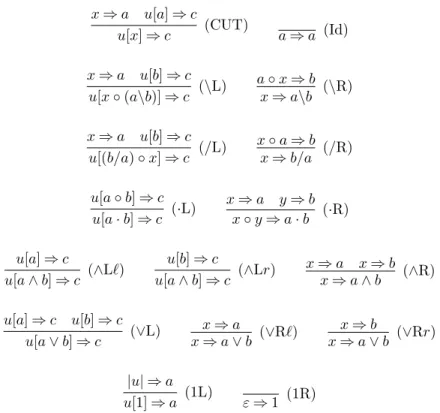
The sequent calculus GL over the language L = {∧, ∨, ·, \, /, 1, 0} is speci-fied by the metarules of Figure 1. Instances of the metarules are obtained by replacing the metavariables a, b, c by formulas over L, the metavariables x, y by groupoid words in (F mL)γ and u by an augmented groupoid word in (F mL)α;
recall that |u| = u[ε]. In what follows we will use GL to refer to both the set of metarules specifying it and to the actual set of rules (instances of the metarules).
With the exception of the first two rules of the system GL, every rule in-troduces a connective to the left or right-hand side of a sequent; depending on the side on which the connective is introduced, we distinguish between left and right rules. Note that the left rules of GL can be simplified in the presence of cut, but we lose the cut elimination property. For example, u[a] in (∨L) can be replaced by groupoid words, where a is a (left or right) outermost formula; to prove the equivalence we use (\R) and (/R).
If R is a set of metarules, not to be confused with the notation used for right rules, then GLR denotes the expansion of GL by the metarules from R.
The system GLfR, called cut-free GLR, is obtained from GLRby removing the
x ⇒ a u[a] ⇒ c
u[x] ⇒ c (CUT) a ⇒ a (Id)
x ⇒ a u[b] ⇒ c u[x ◦ (a\b)] ⇒ c (\L) a ◦ x ⇒ b x ⇒ a\b (\R) x ⇒ a u[b] ⇒ c u[(b/a) ◦ x] ⇒ c (/L) x ◦ a ⇒ b x ⇒ b/a (/R) u[a ◦ b] ⇒ c u[a · b] ⇒ c (·L) x ⇒ a y ⇒ b x ◦ y ⇒ a · b (·R) u[a] ⇒ c u[a ∧ b] ⇒ c (∧L`) u[b] ⇒ c u[a ∧ b] ⇒ c (∧Lr) x ⇒ a x ⇒ b x ⇒ a ∧ b (∧R) u[a] ⇒ c u[b] ⇒ c u[a ∨ b] ⇒ c (∨L) x ⇒ a x ⇒ a ∨ b (∨R`) x ⇒ b x ⇒ a ∨ b (∨Rr) |u| ⇒ a u[1] ⇒ a (1L) ε ⇒ 1 (1R)
Figure 1: The system GL.
2.1.5. Proofs
We define proofs (from assumptions) in GLR, their conclusions and their
(set of ) assumptions by mutual induction.
• A sequent is a proof, whose conclusion and assumption is itself. • A rule s1s2··· sn
s (r) in GLR is a proof, whose conclusion is s and whose
assumptions are s1, s2, . . . sn (more precisely, whose set of assumptions is
{s1, s2, . . . sn}).
• Let Π1, Π2, . . . , Πn be proofs in GLR with conclusions s1, . . . sn,
respec-tively, and sets of assumptions S1, S2, . . . , Sn, respectively. If s1s2s··· sn(r)
is a rule in GLR, then Π1Π2s··· Πn(r) is a proof whose conclusion is s and
whose set of assumptions is S1∪ · · · ∪ Sn.
Metaproofs are defined in a similar way, using the obvious notion for schematic substitution for expressions like u[x]. The following notions have analogues for metaproofs and metasequents, as well.
We say that a sequent s is provable or derivable in GLR from a set S of
whose set of assumptions is contained in S. It is easy to see that `GLR is a
consequence relation on the set of sequents; we will call it the deducibility or provability relation of the Gentzen system.
If s is provable in GLR from an empty set of assumptions, then we simply
say that s is provable in GLR. Proofs from assumptions that have an empty set
of assumptions are simply called proofs.
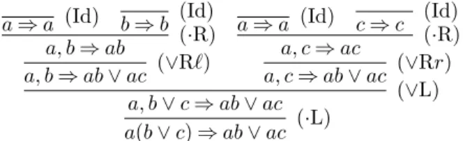
Depending on whether a, b, c are formulas (in FmL) or metavariables for
formulas (in F), the following is an example of a proof or a metaproof in GL.
a ⇒ a (Id) b ⇒ b (Id) a, b ⇒ ab (·R) a, b ⇒ ab ∨ ac (∨R`) a ⇒ a (Id) c ⇒ c (Id) a, c ⇒ ac (·R) a, c ⇒ ab ∨ ac (∨Rr) a, b ∨ c ⇒ ab ∨ ac (∨L) a(b ∨ c) ⇒ ab ∨ ac (·L) 2.1.6. Structural rules
The Gentzen system FL is defined in a way similar to GL. The essential difference is that the left-hand side of an associative sequent is not a groupoid word, but a sequence (a monoid word) of formulas. Augmented associative sequences are associative versions of augmented groupoid words, as well, and the operation ◦ in the definition of metasequents is taken to be associative for associative metasequents; see [36] for more on FL. With the understanding that they are defined over different syntactic objects (sequents), the metarules of the systems GL and FL are the same; the difference lies in the instances of the metarules. Obviously, GL is more expressive than FL and it can be shown that FL is equivalent to a restricted version of GL.
u[(x ◦ y) ◦ z] ⇒ a u[x ◦ (y ◦ z)] ⇒ a (a) u[y ◦ x] ⇒ a u[x ◦ y] ⇒ a (e) u[x ◦ x] ⇒ a u[x] ⇒ a (c) |u| ⇒ a u[x] ⇒ a (i)
0 ⇒ a (o) (w) = (i) + (o)
Figure 2: The basic metarules
Let GLadenote the expansion of GL by the rule (a) of Figure 2; the double
line in (a) means that the metarule can be applied in both directions. Given a sequent, an associative sequent can be obtained by ignoring the parentheses. It can be shown that a sequent is provable in GLaiff the corresponding associative
sequent is provable in FL. Actually, GLa is equivalent to FL in the sense of
We refer to the rules of Figure 2 as (global) associativity, exchange, con-traction, integrality or left weakening, and right weakening; we also refer to the combination of (i) and (o) as weakening and we denote it by (w). We call these metarules basic. Note that our basic metarules are different than the ones usu-ally considered. For example exchange is usuusu-ally written with the metagroupoid words x, y ∈ X replaced by b, c ∈ F, respectively. This means that in its appli-cation only formulas can be commuted while commutation of groupoid words is not assumed; we use boldface (e) for this restricted version of the ‘global’ metarule (e). These rules can also be applied to FL, yielding the systems FLe
and FLe. It can be shown that these two systems have exactly the same
de-ducibility relation; the same holds for FLfe and FLfe. Nevertheless, even though FLc and FLc have the same deducibility relation, the systems FLfc and FL
f c
do not. Therefore, it matters whether the metarules refer to groupoid words or formula metavariables. As for the case of GLa and FL, the systems GLR∪{a}
and FLRare equivalent, for every set R of metarules. In particular, GLaecw is
equivalent to Gentzen’s original system LJ for intuitionistic logic.
Observe that the basic metarules do not involve any connectives; metarules with this property are called structural. Basic metarules are special cases of what we will call simple structural metarules. Recall the formal definition of a metarule from Section 2.1.3, as well as the special meaning of the sets F, A, X, U. A metagroupoid word (a term of sort SX) t that involves only ◦ (and not ?) and
only metavariables from X (not from A) will be called simple. In other words, simple metagroupoid words are groupoid words over the set X of metavariables. For example, (x ◦ y) ◦ x is such a term, for x, y ∈ X. Fix metavariables u ∈ U and a ∈ F. If t0, t1, . . . , tn are simple metagroupoid words and t0 is linear (every
metavariable occurs once), the metarule
u[t1] ⇒ a · · · u[tn] ⇒ a
u[t0] ⇒ a
(r)
is called simple.
2.1.7. Decidability and cut elimination
As mentioned above, a is a theorem of intuitionistic logic iff `GLaecw ε ⇒ a.
Therefore, deciding theoremhood in intuitionistic logic reduces to deciding prov-ability in GLaecw. Note that with the exception of (a), (e), (c) and (CUT), all
the rules reduce the complexity of a sequent as we search upwards for a proof. Rules (a) and (e) rearrange the formulas in the sequent and can be responsible for an infinite loop in the proof search, but with their careful application this effect can be controlled without changing provability. The same can be done, with much more care, for the rule (c) that otherwise increases the complexity as we search upwards; see [34] for details. The rule (CUT) causes considerably more complications as it introduces a new formula. Nevertheless, the system ob-tained from GLaecwby removing (CUT) has the same provable sequents as the
original one (this holds only for provability without assumptions) and this is the content of the cut-elimination property originally established by Gentzen. Cut
elimination has been established by proof-theoretic methods for all the systems GLR, where R is a set of basic rules, see [34], [14]; it is important that we select
the global versions of the simple structural rules, as for example FLc enjoys cut
elimination, but FLc does not. We will present a semantical (algebraic) proof
of this fact in Section 4.2.
2.1.8. The external consequence relation
If B ∪ {c} is a set of formulas, and R is a set of metarules, we write B `GLR c
if {ε ⇒ b | b ∈ B} `GLR ε ⇒ c. Note the difference in the position of GLR
(superscript or subscript) in the two relations. It is not hard to see that `GLR
is a consequence relation on F mL, called the external consequence relation of
`GLR. We will show that the consequence relations `
GLR and `
GLR are actually
equivalent in the sense of [22] (see Section 2.2.5 and Appendix A) thus the former can actually be defined in terms of the latter. Moreover, in the next section we will introduce a Hilbert system and prove that the consequence relation associated with it is equal to `GL.
2.1.9. Solvability
Given a deductive system D (for example GL) and a sublanguage K (for example, {∧, ∨}) of the language L used in D, we can consider subsystems of D associated with K. A natural choice for such a subsystem is the set of all the rules of inference of S that involve connectives only from K plus possibly a fixed set (for example {\, /}) of basic connectives. Traditionally, implication is such a basic connective for Hilbert-style systems, since otherwise we would not allow modus ponens. As long as the set of basic connectives contains · and at least one of \ or /, then this notion of subsystem behaves well for GL. For example, the external consequence relation of such a subsystem is equivalent to the consequence relation of the subsystem. Although, such a definition works well for FL, for a smaller set of basic connectives (just {\} or {/}), it needs some fine tuning for GL, so as to yield the desired results (equivalence with the external relation and the associated Hilbert system) for such a small set of basic connectives.
To motivate the definition of a subsystem of GL, we mention the following. In order to prove the equivalence between the deducibility relation of a subsys-tem of GL and its external consequence relation, or the deducibility relation of the corresponding subsystem of the Hilbert system to be introduced, it is necessary to be able to translate (transform) a sequent into a formula. In the presence of · and at least one of \ or /, for x 6= ε, we can translate a sequent x ⇒ a into the formula φ(x)\a or or the formula a/φ(x), where φ(x) is the for-mula obtained from the groupoid word x by replacing all occurrences of ◦ by ·; we translate the sequent ε ⇒ a into the formula a. This works essentially be-cause the sequents x ⇒ a, ε ⇒ φ(x)\a and ε ⇒ a/φ(x) are mutually derivable in (the {·, \, /} subsystem of) GL. If we lack multiplication, the translation is still possible in the case of FL; we simply translate the sequent a1, a2, . . . an⇒ a to
the formula an\ . . . (a2\(a1\a)); note that the order is reversed. Again this works
derivable in (the {\} subsystem of) FL. Unfortunately, because of the lack of associativity, the same is not possible for GL. For example, there is no sequent of the form ε ⇒ f that is mutually derivable with the sequent (a, b), (c, d) ⇒ e in the multiplication-free subsystem of GL. It is, therefore, necessary to iden-tify the actual subsystem of GL whose deducibility relation is equivalent to its external consequence relation.
We define the set of solvable groupoid words inductively: 1. Every element in Q ∪ {ε} is a solvable groupoid word.
2. If x is a solvable groupoid word and a ∈ Q, then x ◦ a and a ◦ x are solvable groupoid words.
For example the groupoid word (a, (((a, b), c), d)) is solvable, but (((a, b), c), (a, b)) is not. Thus, solvable groupoid words over formulas are exactly the ones that can be translated into a formula, namely they are exactly the left-hand sides of sequents that can be solved [by means of the rules (\R) and (/R)] for ε on the left hand side without using multiplication. Note that a, (((a, b), c), d) ⇒ e is solvable into (i.e., mutually derivable in the multiplication-free subsystem of GL with) ε ⇒ ((((a\e)/d)/c)/b)/a. The ‘solution’ is not unique;
ε ⇒ a\((((a\e)/d)/c)/b) and ε ⇒ (a\(((a\e)/d)/c))/b
are solutions, as well, obtained by a different order of application of the rules (\R) and (/R). Nevertheless, ε ⇒ (a\(c\((a\e)/d)))/b is not a solution, as the only freedom is given after the step a, b ⇒ ((a\e)/d)/c. Note that the term tree (the tree associated with a term) corresponding to a solvable groupoid word has a distinct shape; there is a main branch such that only leaves stem out of it.
We define the set of solvable augmented groupoid words over a set Q induc-tively:
1. The constant is a solvable augmented groupoid word.
2. If u is a solvable augmented groupoid word and a ∈ Q, then u ◦ a and a ◦ u are solvable augmented groupoid words.
For example, following two the augmented groupoid words (a, ((( , a), c), d)) and (a, (((b, ), c), d)) are solvable, but (a, (((a, b), ), d)) and (((a, ), c), (a, b)) are not. Thus, solvable augmented groupoid words over formulas are exactly the right hand-sides of (augmented) sequents that can be solved for on the left hand side without using multiplication. Here the solution is unique; for example the unique solution to the augmented sequent (a, (((b, ), c), d)) ⇒ e is the augmented sequent ⇒ b\(((a\e)/d)/c). Here we used the term augmented sequent for a sequent that allows on the left-hand side.
Left solvable (augmented) groupoid words are defined in a similar way, if in (2) we allow only a ◦ x (a ◦ u) to be left solvable. A groupoid word is left solvable iff it is completely associated to the right. For example the groupoid word (a, (a, (a, a))) is left solvable, but ((a, (b, a)), a) is not. The augmented groupoid word (a, (a, (b, ))) is left solvable, but (a, (a, ( , a))) is not. Note that left solvable (augmented) groupoid words are exactly the ones that are solvable
by using only the left division operation \. For example, (a, (a, (b, a))) ⇒ c is left-solvable into ε ⇒ a\(b\(a\(a\c))) and (a, (a, (b, ))) ⇒ c is left-solvable into ⇒ b\(a\(a\c)). Obviously, every left solvable groupoid word is solvable. Likewise, we define right solvable (augmented) groupoid words.
We also define product left solvable augmented groupoid words, by modifying condition (2) to: If u is a product left solvable augmented groupoid word and x ∈ Qγ, then x ◦ u is product left solvable.
According to the connectives needed for solving a groupoid word, the latter is called fit with respect to the corresponding connectives. More precisely, let K be a sublanguage of L that contains at least one of the connectives \ and /. An (augmented) groupoid word x is called fit for K or an (augmented) K-groupoid word, if it involves only connectives contained in K and the following conditions are satisfied:
1. If K does not contain ·, then x is solvable.
2. If K contains neither · nor /, then x is left solvable. 3. If K contains neither · nor \, then x is right solvable. 4. If K contains ·, but not /, then x is product left solvable.
For example, ((((p ∧ q\p, p), q ∧ p), p), q) is fit for {\, ∧, /}, but not for {\, ∧}. Also, (((p ∧ q\p, p), q ∧ p), (p, q)) is fit for {\, ∧, ·}, but not for {\, ∧, /}.
We denote by QγK and QαK the sets of groupoid and augmented groupoid
words over Q fit for K. A sequent x ⇒ a is called fit for K or a K-sequent, if x is a K-groupoid word and a is a K-formula.
As explained above a sequent calculus can be specified by a set of metarules together with a way to obtain their instances; to define the subsystems of GL, we restrict the instances of the metarules of GL. If K is a sublanguage of L that contains at least one of the connectives \ and /, then the K-subsystem KGL of GL is specified by the metarules of GL that do not involve connectives outside of K; the allowed instances of those metarules are ones in which all the resulting sequents are fit for K. For example, the instance
(c, d), (a, f ) ⇒ e (c, d), (a ∧ b, f ) ⇒ e
of the rule (∧L`) is not included in {∧, \, /}GL, because the sequents involved are not solvable and multiplication is not included in the language.
The consequence relations `KGL and `KGL, for different choices of K, are
defined in the obvious way. Recall that if R is a set of metarules, then GLR
denotes the system obtained from GL by adding the set R. If K is a sublanguage of L that contains \, the system KGLR, is obtained by adding to the rules of
KGL all rules that are instances of the metarules in R so that all the resulting sequents are fit for K.
In the case of FL the K-subsystem KFL does not put any restrictions on the instances of the metarules, since in all instances the resulting sequents are fit for a sublanguage K that contains at least one of the connectives \ and /.
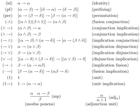
(id) α → α (identity) (pf) (α → β) → [(δ → α) → (δ → β)] (prefixing) (per) [α → (β → δ)] → [β → (α → δ)] (permutation) (·∧) [(α ∧ 1)(β ∧ 1)] → (α ∧ β) (fusion conjunction) (∧ →) (α ∧ β) → α (conjunction implication) (∧ →) (α ∧ β) → β (conjunction implication) (→ ∧) [(α → β) ∧ (α → δ)] → [α → (β ∧ δ)] (implication conjunction) (→ ∨) α → (α ∨ β) (implication disjunction) (→ ∨) β → (α ∨ β) (implication disjunction) (∨ →) [(α → δ) ∧ (β → δ)] → [(α ∨ β) → δ] (disjunction implication) (→ ·) β → (α → αβ) (implication fusion) (· →) [β → (α → δ)] → (αβ → δ) (fusion implication) (1) 1 (unit) (1→) 1 → (α → α) (unit implication) α α → β β (mp) (modus ponens) α α ∧ 1 (adju) (adjunction unit)
Figure 3: The system HL0ae.
2.2. Hilbert systems
In this section we will define a Hilbert-style system HL with deducibility relation equivalent to the relation `GL. The system contains (infinitely) many
rules (schemes) of inference, but it enjoys the strong separation property (with respect to {\}), which states that for every proof only the rules that involve the connectives in the assumptions and the conclusion (and possibly \) are needed in the derivation. In Section 4.5, we present extensions of HL (to the associative, commutative and other cases) which also enjoy the strong separation property; see also Lemma 4.20. We first present simplified versions HL0ae (Figure 3) and HL0a (Figure 4) of HL that correspond to FL and FLe, but do not have the
strong separation property. 2.2.1. The Hilbert system sHL
The Hilbert-style system sHL is an equivalent variant of HL with finitely many rules. It enjoys the strong separation property for signatures that contain ∧ whenever they contain ∨ (Corollary 2.4), but does not have the property for other signatures. We introduce the systems HL0ae, HL0aand sHL before HL,
as the latter is more complicated.
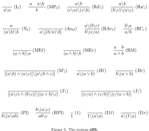
The system sHL is specified by the metarules of Figure 5. To define (Hilbert-style) metarules formally, as before let F be the set (disjoint from the set P of
(id`) α\α (identity) (pf`) (α\β)\[(δ\α)\(δ\β)] (prefixing) (as``) α\[(β/α)\β] (assertion) (a) [(β\δ)/α]\[β\(δ/α)] (associativity) (·\/) [(β(β\α))/β]\(α/β) (fusion divisions) (·∧) [(α ∧ 1)(β ∧ 1)]\(α ∧ β) (fusion conjunction) (∧\) (α ∧ β)\α (conjunction division) (∧\) (α ∧ β)\β (conjunction division) (\∧) [(α\β) ∧ (α\δ)]\[α\(β ∧ δ)] (division conjunction) (\∨) α\(α ∨ β) (division disjunction) (\∨) β\(α ∨ β) (division disjunction) (∨\) [(α\δ) ∧ (β\δ)]\[(α ∨ β)\δ] (disjunction division) (\·) β\(α\αβ) (division fusion) (·\) [β\(α\δ)]\(αβ\δ) (fusion division) (1) 1 (unit) (1\) 1\(α\α) (unit division) (\1) α\(1\α) (division unit) α α\β β (mp`) α α ∧ 1(adju) α β\αβ (pn`) α βα/β (pnr) (modus ponens) (adjunction unit) (product normality)
propositional variables) of formula metavariables and let A be the set of all L-formulas over F. A Hilbert-style metarule is a pair (S, s), where S ∪ {s} is a subset of A. An instance of a metarule is obtained by replacing elements of F by formulas in F mL(P ). a\a (I`) a a\b b (MP`) a\b (c\a)\(c\b) (Rd\) a\b (b\c)\(a\c)(Rn\) a
(a\b)\b (N`) a\[(b/a)\b] (As``)
a\(b\c)
b\(c/a) (RAr`)
b\a a/b (RCr)
(a ∧ b)\a (ME`) (a ∧ b)\b (MEr)
a b a ∧ b (RM)
[(a\b) ∧ (a\c)]\[a\(b ∧ c)] (M\) a\(a ∨ b) (JI`) b\(a ∨ b) (JIr)
[(a\c) ∧ (b\c)]\[(a ∨ b)\c](J\) [(c/a) ∧ (c/b)]\[c/(a ∨ b)] (J/)
b\(a\ab) (PI)
b\(a\c)
ab\c (RPI) 1 (1) 1\(a\a) (I1`) a\(1\a) (I1r)
Figure 5: The system sHL
We note that (I1`) follows from the other rules, but we include it for uni-formity. Indeed, we have (a\a)\[1\(a\a)] by (I1`), and a\a by (I`); then (MP`)
gives 1\(a\a).
If (r) is a simple structural metarule involving the simple metagroupoid words t0, t1, . . . , tn (see Section 2.1.6) then we define the axiom tFm0 L\(t
FmL
1 ∨
· · · ∨ tFmL
n ); here tFmL denotes the formula resulting from t by replacing ◦ by ·.
If R is a set of simple structural metarules, then sHLRdenotes the expansion
of sHL by the axioms corresponding to R.
Given a sequent x ⇒ b, we define the formula φ(x ⇒ b) = φ(x)\b, where φ(x) is the formula obtained by replacing ◦ by · in x; for x = ε, we define φ(ε ⇒ b) = b. If S is a set of sequents we define φ[S] = {φ(s) | s ∈ S}. If a ∈ F mL, we define the sequent s(a) = (ε ⇒ a) and if B is a set of formulas,
we define s[B] = {s(b) | b ∈ B}.
Theorem 2.1. Let S ∪ {s} be a set of sequents, let B ∪ {c} be a set of formulas and let R be a set of simple structural rules. Then
1. S `GLR s iff φ[S] `sHLR φ(s).
2. B `sHLR c iff s[B] `GLR s(c).
3. s(φ(s)) a`GLR s.
4. φ(s(c)) a`sHLR c.
Theorem 2.2. The strong separation property holds for the system sHL, pro-vided that if the language contains ∨, it also contains ∧.
The proofs of Theorems 2.1 and 2.2 are similar to the proofs of Theorem 2.3 (see Appendix A) and Corollary 4.19, and are left to the reader. A result related to Theorem 2.1 on the (weak) separation property was shown in [37] for a Hilbert system equivalent to FLw.
We mention that the rules (MP`) and (N`) are in the current forms because
of the presence of 1. The same applies to (RCr). (As``) is a non-commutative
version of the assertion axiom. Non-commutativity dictates the existence of the rules (N`) and (RCr). (RAr`) is needed because of the absence of associativity.
(Rd\) needs to be stated in a non-axiom form because the corresponding axiom of prefixing implies associativity.
2.2.2. Definable connectives
Since we want the strong separation property to hold (see Section 4.5) for the Hilbert-style system HL we need enough rules for each connective. A main difficulty is presented when a set of connectives under consideration contains ∨, but not ∧. In order for the strong separation property to work for this case we need an infinite set of rules organized in two metarules (RJ\) and (RJ/) (see Figure 6). To express these metarules, we need to introduce a definable connective K, for each set of connectives K. We will introduce the necessary
notation for the definition of HL in this section.
Recall from the discussion on the subsystems of GL that we have a choice on representing the sequent x ⇒ a by either one of the formulas φ(x)\a and a/φ(x). In case that we have exactly one of the division connectives in our sublanguage K together with multiplication, then there is no choice, but if we have both connectives, then we need to be consistent which of the two formulas to consider. Moreover, if x is a solvable groupoid word there are multiple ‘solutions’ involving the division operations in addition to the two formulas mentioned above. Therefore, we fix a representation φK(x ⇒ b) for
the sequent x ⇒ b, relative to the different sublanguages K, and this will be exactly what we will define x Kb as follows.
Let Q be the set of all L formulas over an alphabet that can be either the set P of propositional variables, or the set F of formula metavariables; so Q = F mL(P) or Q = F mL(F) (we will need both cases for discussing rules
and metarules). First we define the depth d(x) of a groupoid word x ∈ Qγ by
induction:
• d(ε) = −1, d(a) = 0, for a ∈ Q, and
Now, given a sublanguage K of L that contains \, and a (meta)sequent x ⇒ b (x ∈ Qγ and b ∈ Q) fit for K, we define x Kb as follows. Here we assume that
if x ⇒ b is a metasequent, then x is simple.
If K contains multiplication, then x K b = φ(x)\b, where φ(x) is the
formula obtained from the groupoid word x by replacing all occurrences of ◦ by ·; for x = ε we define ε K b = b. For example, ((a, (b, c)), ((d, e), f )) {\,·,∧}
g = ((a(bc))((de)f ))\g.
If K does not contain multiplication (and hence x is solvable), then x Kb
is defined by induction on x: • ε Kb = b;
• for a ∈ Q, a Kb = a\b;
• for x, y ∈ Qγ
, (x ◦ y) K b = y K (φ(x)\b) when d(x) ≤ d(y), and
(x ◦ y) Kb = x K(b/φ(y)) otherwise.
Note that in the last case at least one of x, y is in Q. By this definition we give preference to \ relative to /. For example, (a, ((d, e), f )) {\,/,∧} g =
e\(d\((a\g)/f )), not (d\((a\g)/f ))/e.
Note that x K b is always a ‘solution’ of the sequent x ⇒ b. Also, the
outermost element of Q in x Kb is the rightmost of all occurrences of
subfor-mulas of x of maximum depth. Moreover, if K contains neither multiplication nor / (and hence x is left solvable), then x Kb contains neither multiplication
nor /. In general, x Kb is always a K-formula.
We further define u Kb for u ∈ Q and b ∈ Q. We set Kb = b.
• If K contains · and /, u K b is defined by the clauses (v ◦ x) K b =
v K(b/φ(x)) and (x ◦ v) Kb = v K(φ(x)\b).
• If K does not contain ·, but contains /, we have (v ◦ a) Kb = v K(b/a)
and (a ◦ v) Kb = v K(a\b).
• If K does not contain / nor ·, we have (a ◦ v) Kb = v K(a\b).
• If K does not contain /, but contains ·, then u is product left solvable and we define (x ◦ v) Kb = v K(φ(x)\b).
2.2.3. Hilbert-style metarules
In order to introduce a new type of metarules, including (RJ\) and (RJ/), we need to modify the definition of metarules for a Hilbert system. As before, let F be the set (disjoint from the set P of propositional variables) of formula metavariables and let A be the set of all L-formulas over F. Also, let A0 be the set A together with all formal expressions of the form x M b, where x and Mare new symbols and b ∈ A. A Hilbert-style metarule is a pair (S, s), where
S ∪ {s} is a subset of A0. An instance of a metarule is obtained by replacing elements of F by formulas in F mL(P), and all expressions of the form z Mb
by the formulas obtained by replacing M by a sublanguage of L that contains \, and z by a solvable element of (F mL(P))γ that is fit for M.
2.2.4. The Hilbert system HL
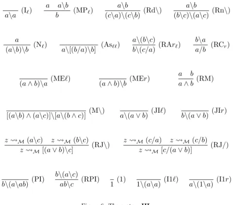
The Hilbert system HL consists of the following metarules, where a, b, c denote formulas; for the rules (RJ\) and (RJ/), M ranges over all sublanguages of L that contain \, and z ranges over all solvable groupoid words over formulas fit for M. a\a (I`) a a\b b (MP`) a\b (c\a)\(c\b) (Rd\) a\b (b\c)\(a\c)(Rn\) a
(a\b)\b (N`) a\[(b/a)\b] (As``)
a\(b\c)
b\(c/a) (RAr`)
b\a a/b (RCr)
(a ∧ b)\a (ME`) (a ∧ b)\b (MEr)
a b a ∧ b (RM)
[(a\b) ∧ (a\c)]\[a\(b ∧ c)] (M\) a\(a ∨ b) (JI`) b\(a ∨ b) (JIr)
z M(a\c) z M(b\c) z M[(a ∨ b)\c] (RJ\) z M(c/a) z M(c/b) z M[c/(a ∨ b)] (RJ/) b\(a\ab) (PI) b\(a\c)
ab\c (RPI) 1 (1) 1\(a\a) (I1`) a\(1\a) (I1r)
Figure 6: The system HL
The de Morgan style axioms (J\) and (J/) of sHL are replaced in HL by the rules (RJ\) and (RJ/), which are important to the proof of the strong separation property (Theorem 2.3).
It is possible to replace some of the rules by the following c ab\a(cb) (N1) c a\[(ab)c/b] (N2) c [a\(ab)c]/b (N3)
However, this simplification destroys the strong separation property, as multi-plication is needed for these rules.
Given a sublanguage K of L that contains the connective \ , the the K-subsystem KHL of HL is defined to be the Hilbert system containing only the rules of HL that involve connectives over K.
The notion of a (meta)proof with assumptions in a Hilbert system is similar to that for sequent calculi. The only difference is that instead of (meta)sequents,
we have (meta)formulas. If a formula c is provable in KHL from assumptions B, then we write B `KHLv.
Also, note that for every sublanguage K of L that contains the connective \ and for every formula a, a a`KHL(a\a)\a; (N`) justifies one direction, and (I`)
and (MP`) justify the other.
A simple structural metarule (r) is called fit for K, if ti is fit for K for every
i. If (r) is fit for K, then we define the Hilbert rule (for a fixed b ∈ F) t1 Kb . . . tn Kb
t0 Kb
h(r)
If R is a set of simple structural metarules, then KHLR denotes the extension
of HL by the rules h(r). 2.2.5. Equivalence
Given a sublanguage K of L that contains the connective \ and a sequent x ⇒ b fit for K, we define the formula φK(x ⇒ b) = x K b. If S is a set of
sequents we set φK[S] = {φK(s) | s ∈ S}.
Recall that if a ∈ F mL, we define the sequent s(a) = (ε ⇒ a) and if B is a
set of formulas, we define s[B] = {s(b) | b ∈ B}.
Theorem 2.3. Let S ∪ {s} be a set of sequents, K a sublanguage of L that contains \, B∪{c} a set of K-formulas and R a set of simple structural metarules fit for K. Then
1. S `KGLR s iff φK[S] `KHLRφK(s).
2. B `KHLR c iff s[B] `KGLR s(c).
3. s(φK(s)) a`KGLR s.
4. φK(s(c)) a`KHLR c.
In the terminology of [22], the theorem states that the two consequence relations are equivalent under the above transformations.
As the proof of Theorem 2.3 is long and would interrupt the flow of the paper we include it, together with the necessary lemmas, in Appendix A (see Corollary A.5).
Corollary 2.4. The results of Theorem 2.3 hold also for sHL in place of HL, for signatures K that contain ∧ whenever they contain ∨.
Proof. It suffices to show that, for signatures that contain ∧ whenever they contain ∨, the rules (RJ\) and (RJ/) can be replaced by the axioms (J\) and (J/).
It is clear that in the presence of ∧ in the signature the rules imply the axioms, by instantiating z = (a\c) ∧ (b\c). For the converse, starting from the axioms and using repeatedly (Rd\) and its companion version (Rd/), which is shown to be derivable (Lemma A.2 in Appendix A), we can obtain
Note that
{[z K (a\c)] ∧ [z K(b\c)]}\{z K[(a\c) ∧ (b\c)]}
is provable by using (RM K), (ME`), (MEr) and (MP`), so by (T`) we get
{[z K(a\c)] ∧ [z K(b\c)]}\{z K[(a ∨ b)\c]}.
Rules (RM K) and (T`) are derived in Lemma A.2 in Appendix A. By a
combination of (ME`), (MEr) and (MP`) we obtain (RJ\).
Theorem 2.5. There is no Hilbert-style system with finitely many rule schemes that is equivalent to HL and has the strong separation property.
Proof. By way of contradiction assume that there is a Hilbert-style system H with finitely many rule schemes that is equivalent to HL and has the strong sep-aration property. Then the same holds for the extension Hi of H by the axiom
a\(b\a). Put differently, the consequence relation `Hi is finitely axiomatizable.
In particular, the {\, ∨}-fragment of `Hi is finitely axiomatizable. However,
Corollary 3.6 of [42] shows that this fragment is not finitely axiomatizable. It is obvious that in HL the role of \ is different than that of /. Nevertheless, if we interchange the roles of the two division operation, by interchanging all occurrences of a\b with b/a, then we obtain rules that are derivable in HL; these rules are called opposite. Recall that a rule is called derivable if the deducibility relation of the system expanded by the rule is the same as the original one. If we include these opposite rules (and axioms) we obtain an equivalent Hilbert system that is symmetric with respect to the two division operations. All the statements, like Theorem 2.3, that we have made for HL and \ hold for the new system with respect to either of the division operations.
2.3. Algebraic presentations of sequent systems
Sequent systems that do not contain ◦ and do not allow an empty left hand side (in other words the left-hand side is always a single formula) are called algebraic. Usually, we write ≤ for ⇒ and we refer to sequents as inequalities. These systems have the advantage that groupoid words can be avoided and they deal only with formulas, so the syntax is much easier to handle.
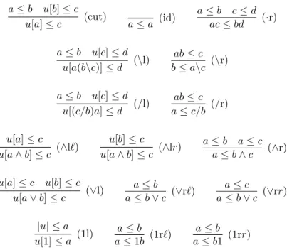
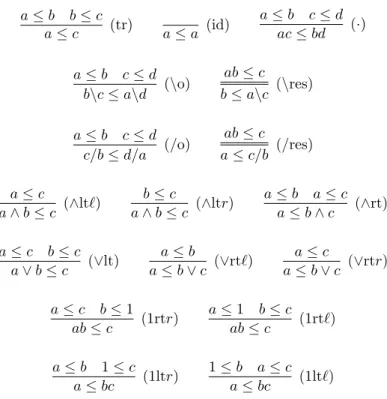
In the following we introduce the algebraic systems PL (Figure 7) and ML (Figure 8) considered in [27] and [26], respectively. Both of them are equivalent to GL and enjoy the cut elimination property. The cut elimination property was established semantically for PL in [27] and using proof theoretic methods for ML in [26]. For more on these systems, see [17]. Computation in PL closely parallels that of GL. On the other hand, ML has two bidirectional rules and is reminiscent of display calculi. The system ML is very convenient for algebraic calculations.
If s is a sequent, we denote by s• the sequent (inequality) resulting from s by replacing ◦ by · and ε by 1. Also, we denote by s◦ the sequent resulting from
a ≤ b u[b] ≤ c
u[a] ≤ c (cut) a ≤ a (id)
a ≤ b c ≤ d ac ≤ bd (·r) a ≤ b u[c] ≤ d u[a(b\c)] ≤ d (\l) ab ≤ c b ≤ a\c (\r) a ≤ b u[c] ≤ d u[(c/b)a] ≤ d (/l) ab ≤ c a ≤ c/b (/r) u[a] ≤ c u[a ∧ b] ≤ c (∧l`) u[b] ≤ c u[a ∧ b] ≤ c (∧lr) a ≤ b a ≤ c a ≤ b ∧ c (∧r) u[a] ≤ c u[b] ≤ c u[a ∨ b] ≤ c (∨l) a ≤ b a ≤ b ∨ c (∨r`) a ≤ c a ≤ b ∨ c (∨rr) |u| ≤ a u[1] ≤ a (1l) a ≤ b a ≤ 1b (1r`) a ≤ b a ≤ b1 (1rr)
Figure 7: The system PL.
s by replacing all external occurrences of · in the left-hand side of s by ◦; here an occurrence of · in a formula is called external if all connectives in the formula tree above the particular occurrence of · are also ·. For example, we replace the inequality (p · q) · [(p · q) ∨ r)] ≤ p · q by the sequent (p ◦ q) ◦ [(p · q) ∨ r)] ⇒ p · q. Theorem 2.6. The systems GL and PL are equivalent. In particular, for every set of sequents S ∪ {s}, and for every inequality ε,
• S `GLs iff S•`PLs•.
• ε a`PL ε◦•.
The same holds for the systems involving fragments of the language that contain multiplication and 1, where the rule instance are restricted appropriately. Proof. If we are given a proof of s in GL from assumptions S, we replace every sequent t by the inequality t• and contract all applications of (·L). Also, the axiom (1R) by an instance of (id). The resulting proof figure is obviously a proof in PL.
Conversely, given a a proof of s in PL from assumptions S, we first replace every inequality t by t◦ in the proof. The resulting proof figure might not be a proof in GL. For example, if an application of the rule (\r) in the original proof has assumption (ab)c ≤ d and conclusion c ≤ (ab)\d, then the translation will yield a rule step with assumption (a ◦ b) ◦ c ⇒ d and conclusion c ⇒ (ab)\d; this is not an instance of the rule (\R), but it is the combination of (·L), which yields
a ≤ b b ≤ c a ≤ c (tr) a ≤ a (id) a ≤ b c ≤ d ac ≤ bd (·) a ≤ b c ≤ d b\c ≤ a\d (\o) ab ≤ c b ≤ a\c (\res) a ≤ b c ≤ d c/b ≤ d/a (/o) ab ≤ c a ≤ c/b (/res) a ≤ c a ∧ b ≤ c (∧lt`) b ≤ c a ∧ b ≤ c (∧ltr) a ≤ b a ≤ c a ≤ b ∧ c (∧rt) a ≤ c b ≤ c a ∨ b ≤ c (∨lt) a ≤ b a ≤ b ∨ c (∨rt`) a ≤ c a ≤ b ∨ c (∨rtr) a ≤ c b ≤ 1 ab ≤ c (1rtr) a ≤ 1 b ≤ c ab ≤ c (1rt`) a ≤ b 1 ≤ c a ≤ bc (1ltr) 1 ≤ b a ≤ c a ≤ bc (1lt`)
Figure 8: The system ML.
(a · b) ◦ c ⇒ d, and of (\R). Therefore, in the proof figure, we insert applications of (·L) before applications of the rules (\R) and (/R), so that x (in these rules) becomes a formula. Likewise, for (1r`) and (1rr), we use (1R) and (·R). Also, for the axioms in the original proof we provide proofs in GL from axioms of the form (Id) applied to formulas. It is not difficult to verify that the resulting proof figure is a proof of s◦ in GL from S◦.
Since ε = ε◦•, the second item of the theorem is clear.
Moreover, the following relation holds between the cut-free systems: `GLf s
iff `PLf s•. The idea is, by moving from bottom upward, in every occurrence of
(\r) and (/r) to replace ab with a ◦ b and propagate this change all the way up in the proof. Moreover, we replace every occurrence of (\l) by an application of (\L) to get u[a ◦ (b\c)] ⇒ d and an application of (·L) to get u[a · (b\c)] ⇒ d; likewise, we modify the occurrences of (/l). Similarly, every application of (·r) is replaced by an application of (·R), followed by an application of (·L). Finally, we replace every occurrence of (1l) by an application of (1L) to get u◦[1] ⇒ d and an application of (·L) to get u[1] ⇒ d; here u◦ is the same as u, except that the · next to is replaced by ◦.
3. Semantical consequence relations
3.1. Residuated lattice-ordered groupoids with unit
A residuated lattice-ordered groupoid with unit or r`u-groupoid, is an algebra L = hL, ∧, ∨, ·, \, /, 1i such that
• hL, ∧, ∨i is a lattice,
• hL, ·, 1i is a groupoid with unit, and
• a · b ≤ c ⇔ a ≤ c/b ⇔ b ≤ a\c, for all a, b, c ∈ L.
We will often assume that the language contains an additional constant 0, of which nothing is assumed. Here ≤ is the order relation associated with the lattice hL, ∧, ∨, i; so, a ≤ b stands for a = a∧b. Note that x/y = max{z |zy ≤ x} and y\x = max{z|yz ≤ x}. The class RLUG of all r`u-groupoids is an equational class; i.e., the class of models of a set of equations. In particular, the identities
x ≈ x ∧ ((xy ∨ z)/y), x(y ∨ z) ≈ xy ∨ xz, (x/y)y ∨ x ≈ x, y ≈ y ∧ (x\(yx ∨ z)), (y ∨ z)x ≈ yx ∨ zx, y(y\x) ∨ x ≈ x. together with the lattice and the unit identities form an axiomatization for it. Consequently, RLUG is a variety; i.e., a class of algebras closed under taking subalgebras, homomorphic images and direct products of the algebras in the class. For basic results and terminology in universal algebra, see [9].
Lemma 3.1. If x, y, yi, where i ∈ I, are elements of a r`u-groupoid and
W yi,V yi exist, then
1. x(W yi) =W(xyi) and (W yi)x =W(yix)
2. (V yi)/x =V(yi/x) and x\(V yi) =V(x\yi)
3. x/(W yi) =V(x/yi) and (W yi)\x =V(yi\x)
4. (x/y)y ≤ x and y(y\x) ≤ x 5. x/1 = x = 1\x
6. 1 ≤ x/x and 1 ≤ x\x.
A residuated lattice, or residuated lattice-ordered monoid, is an associative r`u-groupoid. A residuated lattice is called commutative, if its underlying monoid is commutative. We denote by RL and CRL the varieties of residuated lattices and commutative residuated lattices, respectively. A residuated lattice is commutative iff x\y = y/x for all elements x, y; we denote the common value by x → y.
Lemma 3.2. If x, y, z are elements of a residuated lattice, then 1. x(y/z) ≤ xy/z and (z\y)x ≤ z\yx
2. (x/y)/z = x/zy and z\(y\x) = yz\x 3. x\(y/z) = x\(y/z)
3.2. Logical matrices
Logical matrices are pairs of an algebra and a set and can been used to define logics in the setting of algebraic logic. Here we generalize the standard matrices in two directions. We will generalize the notion of a logical matrix to allow for pairs of a partial algebra and a set. Also, together with the algebra, we will consider a set that is not a subset of the underlying set of the (partial) algebra, but a set of more complex objects.
3.2.1. Multidimensional matrices
We start by reviewing the standard notion of a logical matrix. Recall that if L is a propositional (or algebraic) language, as considered in Section 2.1.2, then an L-algebra is a structure A = hA, (fA)
f ∈Li, where A is a set and for
every f ∈ L of arity α(f ), fA is an operation on A of arity α(f ); we also
write LA or LA for (fA)
f ∈L, and A = hA, LAi. Sometimes, we omit the
superscript A from fA and write A = hA, Li. If L = {f
1, . . . , fn}, we usually
write A = hA, f1, . . . , fni. Also, recall that if A and B are L-algebras, then a
homomorphism from A to B, in symbols h : A → B, is a map h : A → B, such that for every f ∈ L and a ∈ Aα(f ), h(fA(a)) = fB(h(a)), where f (a) = (f (ai))1≤i≤α(f )and h(a) = (h(ai))1≤i≤α(f ), for a = (ai)1≤i≤α(f ).
If P is the set of propositional variables, usually taken to be infinitely count-able, then FmL(P) = hF mL(P), Li is an algebra, called the absolutely free
L-algebra over P or the L-formula L-algebra over P; we often write simply FmL. An
assignment (from FmL(P)) to an L-algebra A is an arbitrary map f : P → A.
Such a map extends uniquely to a homomorphism f : FmL → A.
A (1-dimensional) L-matrix is a pair A = (A, S), where A is an L-algebra and S ⊆ A. The elements of S are called designated or true elements of A. For every subset B ∪ {c} of F mL, we write B |=hA,Si c (or (B, c) ∈ |=hA,Si)
if, for every homomorphism h : FmL → A, h[B] ⊆ S implies h(c) ∈ S, where
h[B] = {h(b) | b ∈ B}. IfM is a class of L-matrices, then |=M is defined to be the intersection of all relations |=A, over all A ∈M. It is easy to see that |=M
is a consequence relation on F mL.
The L-matrix A = hA, Si, is called a matrix model of a consequence relation ` on F mL, if ` ⊆ |=A; in this case S is called a deductive filter for ` (or a
`-filter ) of A. A classM of matrices is called a matrix semantics for a consequence relation `, if ` = |=M. For example, if B is a Boolean algebra and `CPL is
the deducibility relation of Classical Propositional Logic, then hB, {1B}i is a
matrix model of `CPL. It is well known that `CPL = |=h2,{}i, where 2 is the
two-element Boolean algebra. So, {h2, {1}i} and {hB, {1B}i | b ∈ BA}, where
BA is the class of all Boolean algebras, are matrix semantics for `CPL. See [16]
for more on matrices.
Generalizations of 1-dimensional matrices include n-dimensional ones. An n-dimensional L-matrix is a pair A = hA, Si, where A is an L-algebra and S ⊆ An. For every subset B ∪ {c} of (F m
L)n, we define B |=A c iff, for every
homomorphism h : FmL → A, h[B] ⊆ S implies h(c) ∈ S; here h(c) is defined
the same information content with A. If M is a class of n-dimensional L-matrices, the relation |=M is defined in the obvious way. Clearly, |=M is a consequence relation on (F mL)n, or an n-dimensional consequence relation on
FmL.
If A is an L-algebra, then the 2-dimensional L-matrix hA, =Ai, where =A
denotes the equality relation on A, plays a special role and we simply write |=A
for |=hA,=Ai; we refer to elements of (F mL)2as L-equations and to the elements
of =A as true equalities. In detail, if A is an L-algebra and E ∪ {ε0} is a set of
L-equations, then we write E |=Aε0iff for every homomorphism f : FmL→ A,
if f (ε) is true for all ε ∈ E, then f (ε0) is true, as well. Similarly, if K is a class
of L-algebras, we write |=Kfor the relation defined relative to the corresponding
class of matrices.
Another example of 2-dimensional L-matrices are ordered algebras hA, ≤Ai.
The elements of ≤A are called true inequalities.
3.2.2. Sequent matrices
We, now, want to capture the notion of a true sequent over an algebra. The way to do this is to define as a sequent matrix a pair of an algebra A and a set of sequents over A, namely a subset of Aγ × A, designated as true
se-quents. We mention that this notion of a matrix does not fit into the definition of an n-dimensional matrix, because we have an unbounded number of differ-ent dimensions and because n-dimensional matrices presuppose the presence of associativity.
Although this definition completely captures the intended meaning of the terms, we will need it to be more general for technical reasons. For example, we will want to concentrate on only some of all possible sequents, when we discuss a K-subsystem of GL; in this case we will allow only sequents fit for K to be considered. In a different direction, to prove the strong separation property for HL, which will be discussed in Section 4.5, we will need to considerer the set of subformulas of a set of formulas and view it as a partial subalgebra of F mL. The notion of partial subalgebra also appears naturally, when we consider
the application of our results to the finite embeddability property, which will be discussed in Section 4.6.2. Therefore, our definition will need to allow for partial algebras.
Recall that a partial L-algebra is a structure A = hA, (fA)
f ∈Li, where A is
a set and for every f ∈ L of arity α(f ), fA is a partial operation on A of arity
α(f ). A partial map from A to B is a relation f ⊆ A × B, that is functional, i.e. if (x, y), (x, z) ∈ f , then y = z. As usual we write f (x) = y for (x, y) ∈ f ; when there exists a y ∈ B such that (x, y) ∈ f , we say that f (x) is defined and write f (x) ∈ B or x ∈ f−1[B]; if f (x) is not defined, we say that it is undefined. Also, we write f : A * B for a partial map from A to B. A partial operation on A is partial map from a power of A to A.
Let K be a sublanguage of L. A (partial) assignment from FmKto a partial