Deflation in a Neoclassical Growth Model(Mathematical Economics : Dynamic Macro-economic Theory)

Deflation

in

a

Neoclassical Growth

Modell

Noritaka

Kudoh

Graduate SchoolofEconomics, Hitotsubashi University, Kunitachi,Tokyo 186-8601, Japan

1

Introduction

Recent years have witnessed the revival of theoretical studies into monetary policy and the surprising

comeback ofthe liquidity traps anddeflation in academia. In JaPan,the average inflation rate was-0.5% in

the

1995-2000

period. Thestudyof deflation isnolonger atheoreticalcuriosum;deflation is areal economic

issue.

In thispaper, Iconsider deflation in aneoclassical growth model. Thecash-in-advancemonetarymodel

of Lucas-Stokey (1983) is introduced into

an

otherwise standard overlapping generations economy with

productive capital and government debt. The mainpurposeof thisstudyis to address the following question:

how likely it is to observe deflationary (long-run) equilibrium in aneoclassical growth framework? Ifind

that anecessary condition for adeflationary steady state to exist is that theeconomygrowsat apositive

rate. In other words, in contrast to the conventional wisdom, an economy with anegative growth rate

cannot support deflation in thelongrun. In addition,

_asufficient

condition for asteadystateequilibrium

without government deficits to bedeflationaryis that the nominal interest rate is below the growth rate of

the economy.

Recent theoretical studies reveal that howmonetaryandfiscal policiesare conductedisof critical

impor-tance foruniqueness, determinacy, and stability of equilibria. Suchstudy ofmonetary policyin adynamic

general equilibrium framework dates backat least to Sargent and Wallace (1981),who emphasized the

im-portanceofmonetaryandfiscal policyinteractions indetermininginflation rates. The recent revival of the

theory ofmonetary policy is led by Woodford (1994, 1995, 2001), for example, who pushed Sargent and

Wallace’s argument further and popularized the fiscaltheoryof the price level.

Recent theoretical work

on

monetary policymainlyasks whether aparticular monetary-fiscal policy rule

introduces unintendedinstability such as sunspotfluctuations. To the best of my knowledge, there is little

theoreticalattempt in understanding deflation in the context ofdynamicgeneral equilibrium framework. In

the textbook Keynesian framework,

on

the other hand, deflation

or

disinflation caneasily

occur

when the

aggregate demand declines

or

the aggregate supplygoes up. Sincesuchtextbookexplanationis derived from

$1\mathrm{I}$thanktheScimcikaifoundation for financialsupport

数理解析研究所講究録 1264 巻 2002 年 173-187

astatic,sticky priceframework, it isnotclear whetherdeflationthatis obtained is along-runphenomenon.

Thispaperis intended to shedsomelightondeflationary long-runequilibria_{in aneoclassical growth model.}

It isoften documentedthat the standardneoclassical growth modelfails to provide

_atheoretical

_frame

work_{that is consistent with the conventional wisdom thathigh inflationrates}

_are

_{associated with low nominal}

interestrates. In fact, the standard neoclassical growthmodelimpliesthat

an

increasein themoneygrowth

rate drivesinterest rates $\mathrm{u}\mathrm{p}.2$ The textbook Keynesian

IS-LM model,

on

the other hand, is conformedto

the conventional wisdom. This, however, _{is due to the Keynesian presumption that prices}

_are

_sticky

_so

_that

any change in the nominalinterest rate is equivalent to achange in the real rate of the

same

magnitude.

The theoretical framework Ioffer inthispaper is asimpleneoclassicalgrowth modelwithflexiblepricesin

which higher nominalinterestrates reducecapitalandinflation.

For this is an attempt in understanding deflation in aneoclassical growth framework in general, the

specific model Iadopt here deliberately eliminates unnecessarycomplications. Thus, _{Iextend Diamond’s}

(1965)neoclassicalgrowthframeworktoincorporatemoneyandgovernmentbonds. In order to model money

demand in asimple manner, Iadopt the standard cash-in-advancemodel developed byLucas and Stokey

(1983). Althoughthecash-in-advancemodelofmoney is not commonly usedin

an

overlappinggenerations

framework, it provides asimple yet _{powerful tool to study monetary policy issues within aneoclassical}

productioneconomy.

The primary focus of this paper isondeflation as anequilibrium phenomenon. _{This requires amodel}

in which the money growth rate is endogenous. Thus, Iconsider an environment in which the monetary

authority conducts its policy via nominal interest ratepegging. It is shown thatifthegovernment hasno

budget deficits, then there

are

in general two steady state equilibria. The steady state with alow capital

stock has alow inflation rate and is deflationary if the nominalinterestrate is set below thegrowth rateof

theeconomy. _{It is shown that such asteady state is asaddle. The other steady state is associated witha}

highinflationrate, but the real bondholdingat _{that steady state is negative. The steady stateis shownto}

be asymptotically stable.

Iextend the model byintroducinggovernmentdeficits. Introduction ofsuchdeficits changesthe prop

erties of the economy in afew respects. First, there

are

two steady state equilibria, both of which

are

dynamically inefficient. Second, the real bond holdingat both steadystates

can

be positiveif the amount

ofdeficitsissufficientlylarge. Finally, deflationarysteady stateis less likely to

occur

if thegovernmenthas

largedeficits.

$\overline{2\mathrm{S}\mathrm{e}\mathrm{e}.\mathrm{f}\mathrm{o}\mathrm{r}\mathrm{e}\mathrm{x}\mathrm{a}\mathrm{m}\mathrm{p}\mathrm{l}\mathrm{e}.\mathrm{C}\mathrm{h}\mathrm{r}\mathrm{i}\mathrm{s}\mathrm{t}\mathrm{i}\mathrm{a}\mathrm{n}\mathrm{o}\mathrm{a}\mathrm{n}\mathrm{d}\mathrm{E}\mathfrak{i}\mathrm{d}\mathrm{t}\mathrm{e}\mathrm{n}\mathrm{b}\mathrm{a}\mathrm{u}\mathrm{m}}$

$(1092)$.

The rest ofthe paper is organized as follows. Section 2presents asimple budget arithmetic using the

steadystategovernmentbudget constraint. Section3describes the model economy. Section 4characterizes

equilibrium conditions under interest rate pegging. Section 5describes steady state equilibria. Section 6

discusses dynamic properties of the model. Section 7concludes.

2Budget

Arithmetic

Under Deflation

What are the characteristics of an economy that experiences deflation in the long run? In this section

Iconsider implications of deflation for the government’s budget constraint. The flow government budget

constraint is given as

$G_{t}=T_{t}+B_{t}-I_{t}B_{t-1}+M_{t}-M_{t-1}$, (1)

where$G$is the nominalgovernmentspending,$T$is the nominal tax receipt,$B$is the nominalbonds,$M$is the

nominal moneybalance, andI is the grossnominal interest rate. (1) states that government expenditures

arefinanced bytaxes, bonds, and money. Supposethat the economygrowsat thegrossrate of$n>0$

.

Let

$p$denote the price level. Thenone canrewrite (1) as

$g_{t}= \tau_{t}+b_{t}-\frac{R_{t}}{n}b_{t-1}+m_{t}-\frac{1}{\Pi_{t}}\frac{1}{n}m_{t-1}$,

where $g$ is the real government spending per capita, $\tau$ is the real tax per capita, $b$is the real bonds per

capita, $m$is the real money balance per capita, $R$is thegrossreal interest rate,and $\Pi$is thegrossinflation

rate. Suppose thatthere isasteadystateequilibriumin which all per capita real variables

are

constant over

time. Then the steadystate governmentbudgetconstraint is

$g= \tau+(1-\frac{R}{n})b+(1-\frac{1}{\Pi n})m$

.

(2)

Rewrite the government budgetconstraint, using the Fisher equation,$I=R\Pi$_, as

$g= \tau+(1-\frac{I}{\Pi n})b+(1-\frac{1}{\Pi n})m$,

so

thegrossinflation rate is

$\Pi=\frac{Ib+m}{(b+m+\tau-g)n}$

.

(3)

From (3), it is easy to show that, ceteris paribus, $\Pi$ decreases as _$n$ increases. In addition, it is easy to

establish that asteady state is deflationary, orequivalently, $\Pi<1$ holds if and only if

$n> \frac{Ib+7n}{b+m+\tau-g}\equiv\phi$,

In practice, governments

run

positive deficits,

so one can

safely

assume

that $g-\tau\geq 0$

.

Also, the nominal

interest ratecannot be negative. Thus, $\phi$ $>1$ for all $m$ and $b$

.

This implies that $n>1$ must hold

for

a

steady state to _{be deflationary. This supports the conventional view that the growth of the supply side}

causes inflation to go down and may even cause deflation. This implies that for adeflationary long-run

equilibrium to exist,

one

must have amodel which

grows

at apositive rate. Throughout, Iconsider

a

neoclassical gowth model with apositive

exogenous

rateof population growth.

Inow let $n>1$

.

What

are

thecharacteristics of themonetarypolicy underdeflation? Consider

once

again (3). It implies that asteady state equilibriumisdeflationary if and only if

(g$-\tau)n<(n$-I)$b+(n$_-1)m.

In order to obtain sharp result,assumefor

now

that$g=\tau$

.

Then,it follows that in any long-runequilibrium

with$I>1$_{, setting the nominal interest rate at}$I<n$is sufficient for$\Pi$ _$<1$

.

Tosummarize,

Proposition 1 $a$)A necessary condition

for deflation

is that

an

economy

grows at

a

positiverate. $b$)At any

steadystate equilibriumwithoutgovernment deficits, a

_sufficient

condition

_for

_deflation

is that the nominal

interest rate is belcnu the gmwh rate

_of

theeconomy.

Aneconomythat experiencesdeflationis

one

in which the nominalinterestrateis belowthe growth rate

of the economy. This is consistent with the historicalobservationthat deflation

occurs

in

an economy

that

is considered

as

being trapped in as0-called liquidity trap (i.e., theeconomy that hits the lowerboundof

the nominal interestrate),suchastheUSin the 1930’s and Japan in the $1990’ \mathrm{s}$

.

Although the structure presentedinthis section considers only thegovernment budget constraint at

a

steadystate, the analysis reveals thata$\mathrm{n}\mathrm{e}\infty \mathrm{s}\mathrm{a}\mathrm{r}\mathrm{y}$condition foradeflationarysteady state to exist is that

theeconomy growsat apositive rate. In otherwords, incontrast to the conventionalwisdom,

an

economy

with anegative growth rate cannotsupport deflationin the long-run. Further, _{setting the nominal interest}

ratebelow thegrowth rate_{of the economy is sufficient for deflation inaneconomy without deficits. In the}

followingsections,_{Ipresent asimple dynamic general equilibrium model thatsupportsdeflationat asteady}

state and discusses the properties of equilibria with deflation.

3The

Model

3.1

Environment

Consideragrowingeconomy consisting ofan infinite sequence oftwo periodlived overlapping generations,

an initial old generation, and an infinitely-lived government. Let $t=1$, 2,$\ldots$ index time. At eachdate $t$,

anew generation comprised of$N_{t}$ identical members appearswhere $N_{t}$ evolves according to$N_{t+1}=nN_{t}$

.

Iassume that population growth is the only

source

of (exogenous) growth. Each agent is endowed with

one

unit oflabor when youngand is retired when old. In addition,the initial old agents

are

endowed with

$M_{0}>0$units of fiat currency and $k_{1}>0$units of capital.

There is asingle final good produced using astandardneoclassicalproduction function$F(K_{t},L_{t})$where

$K_{t}$ denotes the capital input and $L_{t}$ denotes the labor input at $t$

.

Let $k_{t}\equiv K_{l}/L_{t}$ denote the

capital-labor ratio. Then, output per worker at time $t$ may be expressed

as

$f(k_{t}^{\sim})$ where $f(h)$ $\equiv F(K_{t}/L_{t}, 1)$ is

the intensiveproduction function. Iassume that $f(0)=0$,

$f’>0>f’$

, and that Inada conditions hold.

The final good can either be consumed in the period it is produced, or it can be stored to yield capital

the following period. For

reasons

ofanalytical tractability, capitalis assumed to depreciate lm% between

periods.

3-2

Factor Markets

Factor markets are perfectly competitive. Thus, factors of production receive their marginal product. Let

$r_{t+1}$ denote the gross return on capital, and let $w_{t}$ denote the real wage rate. Young agents supply their

labor endowmentinelastically in the labor market. Then,firms’ profit maximizationrequires

$r_{t+1}$ $=$ $f’(k_{t+1}.)$, (4)

$w_{t}$ $=$ $f(k_{t}.)-k_{t}f’(k_{\mathrm{t}})\equiv w(k_{t})$

.

(5)

Note that $w’(k)=-kf’$$(\ )>0$for all $k$

.

It will be useful to introduce arestriction onthe production

technology. In particular, Iassume throughout that $k.w’(k)/w(k)<1$ holds. Cobb Douglas production

function, forexample,satisfies this condition.

3.3

Consumers

Let $c_{1t}(c_{2t})$ denote the consumption of the final good by ayoung (old) agent born at date $t$

.

In order

to simplifythe analysis as muchas possible, Iassumethat agents careconsumptiononly when old. This

immediately follows that $c_{1t}=0$ for all $t$so aU income $\mathrm{w}\mathrm{i}\mathrm{U}$be saved. Following Lucas and Stokey (1983)

and

more

recently Woodford (1994), Iassume that consumption goods are dividedinto two types: “cash

goods” and “credit goods.” Cash goods must be purchased bycash, so agents wishing to

consume

cash

goods need cash in advance. Onthe otherhand,agentsdo not need cash to purchase credit goods. Let$Cmt$

$(c_{nt})$denote the amount of cash (credit)goods consumed when old. Then,

$c_{2t}=c_{mt}+c_{nt}$ holds. Iassume

that the marginal rate oftransformation inproductionis unitybetweenthe two goodssothe price of the

two goodsis identical and denoted by $P_{t}$

.

Thecash-in-advanceconstraint is

$p_{\mathrm{t}+1}c_{mt} \leq\frac{M_{t}}{N_{t}}$, (6)

whereptdenotes thetime$t$price level and_$Mt/Nt$denotes the nominalmoneybalance peryoung,

According

to (6),

ayoung

agent mustset aside cash in advance in order topurchasecashgoods when old.

It is assumed that agentsmay hold moneyand non-monetary assets. Thenon-monetaryassets,denoted

by$A_{t}$,

are

assumed to yield the grossnominal return of_{$I_{t+1}\geq 1$}

in the next period. Iassumethat agents

do nothave

access

toany otherstoragetechnology. The budget constraint forayoungagent born at date

$t$istherefore

$\frac{M_{l}}{N_{t}}+\frac{A_{l}}{N_{t}}\leq p_{t}w_{t}$, (7)

where$A_{t}/N_{t}$ is the non-monetary asset holding per capita. (7) states that

ayoung

_{agent of generation}

$t$

receives nominal wage incomeand allocates all incometo monetary and non-monetary assets (because

no

one

consumes

whenyoung). _{Throughout, Iconsider only symmetric equilbria in which all agents of the}

same

generation have the

same

amount of assets. Sincethe nominal interest rate

on

money is zero, the budget constraint when old is

$p_{\ell+1}c_{2t} \leq\frac{M_{t}}{N_{t}}+I_{t+1}\frac{A_{t}}{N_{t}}$

.

(8)

Divide both sides of(7) and (8) by$pt$ and$p_{t+1}$

.

respectively, toobtain

$m_{t}+a_{t}\leq w_{t}$ ₍₉₎

and

$c_{2t} \leq\frac{p_{t}}{p_{t+1}}m_{t}+R_{t+1}a_{t}$, (10)

where$m_{t}\equiv M_{t}/N_{t}p_{t}$, $a_{t}\equiv A_{t}/N_{t}p_{t}$, andthegrossrealinterest ratesatisfies

the Fisher equation,

$I_{t+1}\equiv R_{t+1^{\frac{p_{C\dagger 1}}{p\iota}}}$

.

(11)

Individualrationality implies that (9) and (10) hold at equality. Eliminate $a_{t}$ from (9) and (10) to obtain

theintertemporal budget constraint,

$\frac{c_{2t}}{R_{t+1}}+\frac{I_{t+1}-1}{I_{t+1}}m_{t}=w_{t}$

.

(12)

The cash-in-advance constraint binds if andonlyif money is dominatedby non-monetaryassets in rates

ofreturn, which is equivalent to $I_{t+1}\geq 1$

.

In otherwords, the cash-in-advance constraint binds

as

longas

the nominalinterest rate is non-negative, which is plausible. Under biding cash-in-advanceconstraint, (6)

holds at equality. Then, (6) and (10) imply that

$c_{mt}$ $=$ $\frac{p_{t}}{p_{t+1}}m_{t}$, (13)

$c_{nt}$ $=$ $R_{t+1}a_{t}$ (14)

must hold in equilibrium.

Following Chari, Christiano, and Kehoe (1991), Ispecify theutilityfunction$\mathrm{a}\mathrm{s}^{3}$

$U$ $(c_{mt}. c_{nt})$ $=$ $\ln c_{t}$, (15)

$c_{t}$ $\equiv$ $[(1-\sigma)c_{mt}^{1-\rho}+\sigma c_{nt}^{1-\rho}]\overline{1}\overline{\rho}\underline{1}$ (16)

where $0<\sigma<1$ and $0<\rho<1$. Each youngagent chooses $Cmt$ and$Cnt$ to maximize (15) subject to (9),

(13), and (14). This problem isequivalent to maximizing

$\ln\{[(1-0)$ $( \frac{p_{C}}{p_{t+1}}m_{t})^{1-\rho}+\sigma(R_{t+1}a_{t})^{1-\rho}]\overline{1}-\rho \mathrm{L}\}$

withrespectto$m_{t}$ and$a_{t}$ subjectto (9). The first order necessary condition for the maximization problem

gives the real money demand function,

$m_{t}=\gamma(I_{t+1})w_{t}$, (17)

where

$\gamma(I)\equiv[1+(\frac{\sigma}{1-\sigma})^{\rho}I^{\underline{1}-A}[perp]\rho]-1$ (18)

It isimportant tocheck the properties of the money demand function just derived.

Lemma 27(I)

_satisfies

(a)$\gamma’(I)<0$

for

_$0<\rho<1$, (b)$\lim_{Iarrow\infty}\gamma(I)=0$

for

_$0<\rho<1$, (c)$0<\gamma(I)<1$,

and (d)

$\frac{I\gamma’(I)}{\gamma(I)}=-\frac{1-\rho}{\rho}[1-\gamma(I)]’$

.

$3\mathrm{A}\mathrm{c}\mathrm{c}\mathrm{o}\mathrm{r}\mathrm{d}\mathrm{i}\mathrm{n}\mathrm{g}$ to Chari, Christiano, and Kchoc (1991), $\sigma=0.57$,$\rho=0.17$ for the

$\mathrm{U}.\mathrm{S}$. economy. Note, however, that the

parameter valuesare for their model economy in which there is an infinitelylived agent, ratherthan aseriesofoverlapPin

179

Proof. SeeKudoh(2001). $\blacksquare$

Lemma2(a) states the condition under which the real

money

demand is decreasing in the nominal

interest rate. As the nominal interest rate increases, the

household

substitutes

away

from

money,

which

reduces money demand. An increase in the nominal rates, at the

same

time, raises earning from bond

holding, which raisesmoneydemand throughincomeeffect. The former dominates the latter if$0<\rho<1$,

whichIassumeto hold throughout. Inaddition, Iassumethat $(1-\rho)I<1$ _{holds, which is plausible and}

easilysatisfied.

It isimportant tocomparecompeting models ofmoney demand inadynamic general equilibrium

envi-ronment. Schreft andSmith $(1997, 2000)$ develop

an

environmentin which spatialseparation and limited

communicationgiverise tothe role ofbankingsectorin providing$1\mathrm{i}\mathrm{q}\mathrm{u}\mathrm{i}\mathrm{d}\mathrm{i}\mathrm{t}\mathrm{y}^{4}$

.

Asis clear, the

money demand

function obtained inthis

paper

is virtually identicaltothe

one

obtained in

Schreft

andSmith $(1997, 2000)$

.

That is, the cash in advance model of Lucas Stokey (1983) and the random relocations model of

Schreft-Smith (1997, 1998, 2000)

are

qualitatively the

same.

An advantage of the present approach is its simple

modelenvironment.

3.4

Monetary and Fiscal

Policy

Rules

Recent theoretical studies of monetary policy reveal that how fiscaland monetary policies

are

conducted

is of crucial importance fordeterminacy,multiplicity, and stabilityof$\mathrm{e}\mathrm{q}\mathrm{u}\mathrm{i}\mathrm{h}.\mathrm{b}\mathrm{r}\mathrm{i}\mathrm{a}^{5}$

.

In thispaper, Iconsider

monetary andfiscalpolicy rules that

are

simple yet plausible. Inparticular,

Iassume

that the fiscal authority

sets thesequenceof the realprimary deficits percapita,and that themonetary_{authority conducts its policy}

through targeting the nominalinterest rate.

To simplify matters, Ilet $T_{t}=0$ for all $t$

.

Then, from (5) the government’s

flow budget constraint becomes

$G_{t}+I_{t}B_{t-1}=B_{t}+M_{t}-M_{l-1}$ ₍₁₉₎

for $t\geq 2$ and $G_{1}+M_{\mathrm{O}}=kI_{1}+B_{1}$ for _$t=1$, where _{the initial stock ofbonds is assumed to bezero.}

I

assume

that thegovernmentsimply

consumes

$G_{t}$ and that it docsnotaffect utility ofanygeneration

or

the

production process at any date. In order to simplify the analysis, Ifurther

assume

that $G_{\iota}/\mathrm{A}_{l}’p_{l}=g\geq 0$

$\overline{\triangleleft \mathrm{W}\mathrm{a}11\mathrm{a}\mathrm{c}\mathrm{e}(1984)\mathrm{a}\mathrm{n}\mathrm{d}\mathrm{B}\mathrm{h}\mathrm{a}\mathrm{t}\mathrm{t}\mathrm{a}\mathrm{c}\mathrm{h}\mathrm{a}\mathrm{r}\mathrm{y}\mathrm{a}\mathrm{a}\mathrm{n}\mathrm{d}1’\backslash \mathrm{u}\mathrm{d}\mathrm{o}\mathrm{h}}$

$(2001)$arc_{examples of the modelin which money isheld bythe banking}

sectorjustto meetthe legalreserverequirement.

$Thestudyofmonetary-fiscal policyinteractions_{in adynamic general equilibrium setup datesbackatleasttoSargentand} Wallace(1981), whofirst linkedmonetary andfiscalpolicies by asinglegovernment’s_{budget constraint. Examples ofrecent}

theoreticalworkonmonetaryPolicy include Lccpcr(1991),Woodford (1994. 1995),andSchmitt-GrohcandUribc (2001).

for all$t$

.

That is,the real government spendingper young is assumed to be constant

over

time. Then, it is

easy to rewrite (19)

as

$g+ \frac{R_{t}}{n}b_{t-1}=m_{t}-\frac{p_{t-1}}{p_{t}}\frac{1}{n}m_{t-1}+b_{\iota}$, (20)

where $b_{t}\equiv B_{t}/N_{tPt}$

.

The absence ofarbitrage opportunityin the capitalmarketrequires that capital and

bondsyield thesamerateofreturn. Thatis, $r_{\ell+1}=R_{t+1}$ holds. Therefore,Ilet$R_{t+1}$ denote the grossrate

of returnon capital, bonds andnon-monetary asset (at) interchangeably.

The primary interest of thispaperisdeflation

as

anequilibrium phenomenon. For this reason, themoney

growth rate and the

inflation

rate must beendogenous in the model. In order todescribe determination of

the inflation rate inasimplemanner, Iassume that themonetary authorityconducts its policy via nominal

interest rate pegging. That is, Iassumethat$I_{t}=I>1$ for all dates.

4Equilibrium

This section characterizes equilibrium conditions of the model.

Definition 3A monetary equilibrium is a set

_of

seqegences

_for

allocations $\{m_{t}\}$, $\{a_{t}\}$, $\{k_{t}\}$, $\{b_{t}\}$, prices

$\{r_{t}\}$, $\{w_{t}\}$, $\{\mathrm{p}\mathrm{t}\}$, and the initial conditions $M_{0}>0$, $k_{1}>0$, $B_{0}=0$ such that (a)

factor

markets clear,

$i.e.$, (4) and (5) hold, (b) assetmarket clears: $IC_{t+1}+N_{t}b_{t}=N\mathrm{t}a\mathrm{t}$, (c) the allocations solve agents’ utility

maximization problem, (d) the cash-in-advance constraint (6) binds,

or

equivalently, $I_{t}>1$ holds, (e) the

government’s budget constraints$g+\mathrm{A}I_{0}=M_{1}+B_{1}$

for

$t=1$ and (19)

for

$t\geq 2$ hold, and (f) $I_{\iota}=I$ and

$g_{t}=g$

for

all$t$

.

Themoney market equilibrium requires that

$\frac{M_{t}}{p_{t}}=\gamma(I)w(k_{t})$

.

(21)

The asset market equilibrium requires$k_{t+1}+b_{t}=a_{t}=w(\mathrm{a}\mathrm{t})-m_{t}$, whichcanbe rewritten

as

$k_{t+1}.+b_{t}=[1-\gamma(I)]w(k_{t}.)$

.

(22)

The Fisher equation implies that thegrossinflation rate is determined by

$\frac{p_{t+1}}{p_{t}}=\frac{I}{f’(k_{t+1})}$

.

(23)

Substitute (23) and (21)into (20) to obtain

$b_{t}=g+ \frac{f’(k_{t})}{n}b_{\ell-1}-\gamma(I)w(k_{t})+\frac{f’(k_{t})}{nI}.\gamma(I)w(k_{t-1}.)$

.

(24)

(22) and (24) describethe laws of motion forcapitaland bonds

5Steady

State

Equilibria

5.1

Existence

Thissectionconsiderssteadystate equilibriain which thegovernmenthasnoprimary deficits, thatis,g$=0$

.

From(22) and (24),steady state equilibria must satisfy

$b=[1-\gamma(I)]w(k)-k\equiv\Gamma(k)$ ₍₂₅₎

and

$b=- \frac{1-\Delta^{k}4\mathfrak{n}I}{1-\angle 1^{k}4,n},,\gamma(I)w(k)\equiv H(k)$

.

(26)

It is important to establish the shape of the function$H$, which is spelt out below.

Lemma 4Let$k_{g}$

.

solve $f’(k)=n$ and letkb solve $f’(k)=nl$

.

Then, the

function

H

satisfies

(a) H_$(0)=$

H$(k_{b})=0$, (b)H$(k)>0\dot{\iota}f$and only

if

$k_{b}<k<k_{\mathit{9}}$

.

(c) $\lim_{karrow k_{l}}.H’(k)=\infty$

.

Proof. Omitted. $\blacksquare$

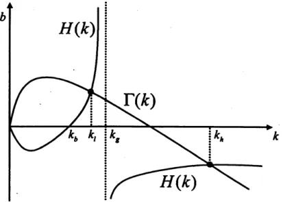
Giventhe shapeof$H$, it iseasytoshowthat steady state equih.bria characterized _{by(25)and (26),}

_are

shown in figure 1. Lemma4, combined with figure 1, implies that there

are

in general two non-trivial steady

stateequilibria.

One

is located in the region$k_{b}.<k<k_{g}$.and $b>0$holds at that steady state. The other

one

isfound in the region$k_{\mathit{9}}<k$ and$b$is negative at that steady state.

Notethatany steady state solves

$k=[1 -\gamma(I)]w(k)-H$(&)\equiv \Omega (k). (27)

For futurereference, it isimportant to knowsomeproperties of the function$\Omega$

.

Lemma

_5Define

$h(I)\equiv 1-\gamma(I)+\gamma(I)/I>0$

.

$Thm$, the

function

$\Omega$

satisfies

(a)

$\Omega(k)=[1-h(I)\frac{f’(k)}{n}]\frac{w(k)}{1-\angle L^{k}\mathit{1},n},$

.

,,

and (b)$\Omega’(k)<1$ holds atany steady state.

Proof. SecKudoh(2001). vi

Lemma 6Let$k_{I}$ solve $f’(k)=I$

.

Then, anysteadystate with _{$k<k_{I}$}

satisfies

_$\Pi<1$

.

Proof. Fromthe Fisher equation, it is easyto showthat$\Pi=I/f’(k)$

.

Thus, $\Pi<1$ holds ifandonlyif

$f’(k)>I$

.

ss

The expression for the steady state inflation rate isobtainedfrom (20)

as

$\Pi=\Pi(k)\equiv,\frac{\gamma(I)w(k)/n}{(1-\angle[perp] k\lrcorner)nb+\gamma(I)w(k)}$

.

Proposition 7A necessary condition

_for

$\Pi<1$ ata steady state etyith $b>0$ is $n>1$

.

Proof. It iseasyto show that

$\Pi<1\Leftrightarrow n>\frac{\gamma(I)w(k)+f’(k)b}{b+\gamma(I)w(k)}\equiv$$($&,$b)$

.

$\phi$(20) $>1$since$f’(k)>1$ at asteady state with$b>0$

. ss

Proposition

_8If

$I<n$ holds at asteadystate equilibrium with$g=0$ and$b>0$, then such asteadystate

isunique andis deflationary.

It is easy to

see

that in the model with$g=0$ and $I<n$, any non-trivial steady state is considered

as

beingindeflation. In otherwords, if themonetaryauthority sets the net nominal interest rate close to zero,

thenthe economy is necessarily deflationary.

Example 9Suppose that the production

_function

is $3k^{0.33}$, and let $\sigma=0.6$, _$\rho=0.2$, $n=1.03$, _$g=0$,

$I=1.\mathrm{O}1$

.

Then, there are two non-trivial steady states at $k_{l}=0.94$, $k_{h}=2.85$

.

The associated

inflation

rates and real bond holdings are, respectively, $\Pi_{\{}=0.98$, $\Pi_{h}=2.05$

,

$b\iota$ $=0.80$, $b_{h}=-0.32$

.

The aboveexample computes steadystate equilibria when$I<n$

.

It demonstrates that thereareindeed

twosteadystate equilibriaand that the low-A;steady state is deflationary.

5.2

Comparative

Statics

Itis

now

possible to studythe effects ofachange in I

on

capitalaccumulationandinflation.

Lemma 10 $h’(I)<0$ holds.

Proof. SeeKudoh (2001). In

Proposition 11

$\frac{dk}{dI}.|_{k=k_{\mathfrak{l}}}.<0$, and $\frac{dk}{dI}|_{k=k_{h}}.>0$

Proof. Totallydifferentiate(27) toobtain

$\frac{dk}{dI}$

.

$=, \frac{-h’(I)\angle_{\mathfrak{n}}k\coprod w(k)}{(1-\angle[perp] k4)n(1-\Omega’(k))}$

.

From Lemma5, $\alpha$$(k)-1<0$ holds atany steady state. Further,From

lemma 10, $h’(I)$ $<0$ holds. _{It is}

therefore easy to establish that $dk/dl<0$if andonlyif$f’(k.)>n$

.

The rest of theproofis immediate. $\blacksquare$

Proposition 11 asserts that

an

increase in the nominal interest rate reduces thecapitallabor ratio if and

onlyif the economy is dynamically efficient at the steady state. Since $k$ and $\Pi$

are

positively related,

an

increasein the nominalinterestratereduces theinflationrate atadynamicallyefficientsteadystate.

Since

anysteadystateequilibrium with$b>0$isdynamicallyefficientinthe model withoutgovernmentdeficits, it

is possible to conclude that atightmoney policy through interest rate targeting reduces capital stock and

inflation in the long

run.

An increase in I reduces the real money balance, which, ceterisparibus, raises

capitalstock. At the

same

time,

an

increase in I raises thedemandfor bonds because the return

on

bonds

goesup. At the low-fc steadystate, the latter effectdominatestheformer

so

capitalinvestment is reduced

andsois inflation.

The result obtained here is consistent with the conventional wisdom that high nominal interest rates

reduceinflation. In fact, the textbook IS-LMmodel predicts that

an

increase in the nominal interest rate

raises the cost ofcapital andreduces investment, which has anegative impact

on

theaggregate

income

and

theinflationrate. Suchpredictions

are

based upon the Keynesian presumption that the price level is sticky.

It is easyto

see

that changes inthe nominal rates

cause

$\mathrm{o}\mathrm{n}\triangleright \mathrm{t}\infty$

-one

changes inthe real ratesundersticky

prices. It iswell-known, however,that getting suchpredictionsinaneoclassical,flexiblepriceframeworkis

not atrivial matter. As Christianoand Eichcnbaum (1992)note, the standard dynamic general equilibrium

model predicts ingeneralthat the growth rateof moneyis positively related with the nominalinterest rate.

Proposition 12 $dk/dn<0$ _{holds at any}steadystate.

Proof. SeeKudoh(2001). $\blacksquare$

Proposition 12 asserts that

an

increase in the growth rate of the economy reduces the steady state

capital-labor ratio and theinflation rate. This result supports the conventional wisdom thatthe capacity

growth

causes

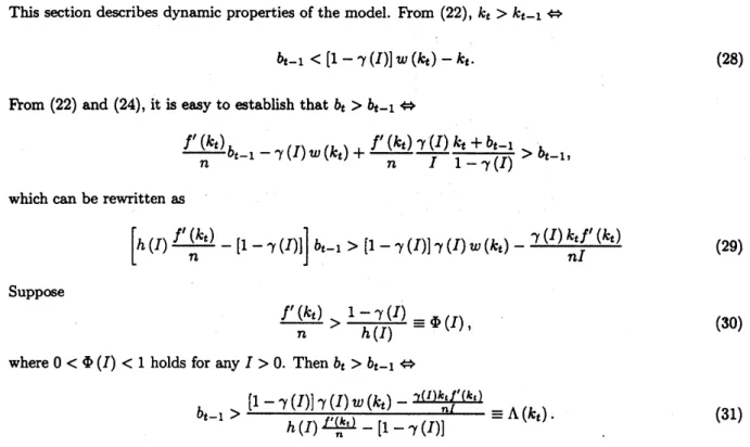
inflation togodown

6Dynamics

This section describesdynamic propertiesof the model. From (22), $k_{t}>k_{t-1}\Leftrightarrow$

$b_{t-1}<[1-\gamma(/)]w(\mathrm{k})-k_{t}$

.

(28)

From (22) and (24), itis easyto establish that$b_{\mathrm{C}}>b_{t-1}\Leftrightarrow$

$\frac{f’(k_{t})}{n}b_{t-1}-\gamma(I)w(k_{t})+\frac{f’(k_{t})}{n}\frac{\gamma(I)}{I}\frac{k_{t}+b_{t-1}}{1-\gamma(I)}>b_{t-1}$,

which

can

berewritten

as

$[h(I) \frac{f’(k_{t})}{n}-[1-\gamma(I)]]b_{t-1}>[1-\gamma(I)]\gamma(I)w(k_{t})-\frac{\gamma(I)hf’(k_{t})}{nI}$ (29)

Suppose

$\frac{f’(k_{t})}{n}>\frac{1-\gamma(I)}{h(I)}\equiv\Phi$$(I)$, (30)

where$0<\Phi$_$(I)<1$ holds forany_$I>0$

.

Then $b_{t}>b_{t-1}\Leftrightarrow$

$b_{t-1}$ (31)

Figure2shows typicalconfiguration of thephasediagram of thesystem,where Ilet$k_{\Phi}$solve$f’(k)=n\Phi$_$(I)$

.

According to figure 2, the low-A; _{steady state is} asaddle, while the high-/: steady state is asymptotically

stable.

7Conclusion

This paper has considered equilibria with deflation in aneoclassical growth model. The cash-in-advance

monetarymodel ofLucas Stokey(1983)isintroducedinto astandardoverlapping generations

economy

with

productive capital and government debt. Monetary policy is conducted via interest rate targeting

so

the

inflation rate is endogenous. In contract to the standard monetary growth model with

an

infinitelylived

agent, the model developedin this paperpredictsthat higher nominal interest rates reduce inflation in the

long-run. Thisprovesthat the model developed in thispaperis areasonable platform for studying monetary

and fiscal policy issues.

Simple budget arithmetic reveals that the necessaryconditionfor along-runequilibrium withdeflation

toarise is that theeconomy grows at apositive rate. Further, ifthe nominal interestrate isset below the

growth rate of theeconomy, then theeconomywithout deficits isdeflationary

Figure 1. Steady state equlibria withoutdeficits.

Figure2. Dynamicalequilibriawithout deficits.

References

[1] Azariadis, Costas. IntertemporalMacroeconomics, Basil Blackwell: NewYork, (1993

[2] Bhattacharya, Joydeep, and Noritaka Kudoh. “TightMoneyPolicies and InflationRevisited”, Canadian

Journal

_of

Economics,forthcoming.

[3] Chari, V. V., Laurence J. Christiano, and Patrick J. Kehoe. “Optimal Fiscal and Monetary Policy:

Some Recent Results.” Journal

of

Money, Credit, and Banking 23 (1991)

519539.

[4] Christiano, Laurence J., and Martin Eichenbaum. “Liquidity Effects and the Monetary Transmission

Mechanism.” American Economic Review AEA Papers andProceedings (1992)

346353.

[5] Diamond, Peter. “National Debt in aNeoclassical Growth Model.” American Economic Review55

(1965)

112650.

[6] Kudoh, Noritaka. “Deflation in aNeoclassical GrowthModel.” Hitotsubashi University, mimeo(2001)

[7] Leeper, Eric. “Equilibria under‘Active’ and ‘Passive’ Monetary and FiscalPolicies,” Journal

_of

Mon-etaryEconomics 27 (1991) 129-147.

[8] Lucas, Robert, and Nancy Stokey. “Optimal Fiscal and Monetary Policyin

an

Economy without Cap

ital,” Journal

_of

MonetaryEconomics

12

(1983)

5593.

[9] Sargent, Thomas J., and Neil Wallace. “Some Unpleasant Monetarist Arithmetic.” Federal Reserve

Bank

_of

Minneapolis Quarterly Review (1981) 1-17.

[10] Schmitt-Grohe, Stephanie, and Martin Uribe, “PriceLevel Determinacyand Monetary Policyundera

Balanced-Budget Requirement,” Journal

of

Monetary Economics45(2000) 211-246.

[11] Schreft, Stacey L., andBruce D. Smith. “Money, Banking, and Capital Formation.” Journal

of

Ec0-nornic Theory 73 (1997) 157-182.

[12] Schreft, Stacey, and BruceSmith. “TheEvolution ofCashTransactions: SomeImplications for

Mone-tary Policy,” Journal

_of

Monetary Economics 46 (2000)

97-120.

[13] Wallace, Neil. “Someof theChoices for Monetary Policy,” Federal Reserve Bank

_of

Minneapolis

Quar-terlyRevi ew (1984)

[14] Woodford, Michael. “Monetary Policyand Price-Level Determinacy in aCash-in-Advance Economy,”

Economic $Theo\eta$ 4 (1994) 345-380.

[15] Woodford, Michael. “Price-Level Determinacy Without Control aMonetary Aggregate,”

Carnegie-Rochester

_Conference

Series on Public Policy 43 (1995) 1-46