A Numerical Simulation Study of Data-driven Pole Placement

A Numerical Simulation Study of Data‑driven Pole Placement

著者 ピョン イ イ シュェ

著者別表示 Pyone Ei Ei Shwe journal or

publication title

博士論文要旨Abstract 学位授与番号 13301甲第4624号

学位名 博士（工学）

学位授与年月日 2017‑09‑26

URL http://hdl.handle.net/2297/00049548

doi: 10.4236/ica.2017.83011

Dissertation Abstract

A Numerical Simulation Study of Data-driven Pole Placement

Division of Electrical Engineering and Computer Science Graduate School of Natural Science & Technology

Kanazawa University

Student Number: 1424042018

Pyone Ei Ei Shwe

Supervisor: Prof. Shigeru YAMAMOTO

1 Abstract

This dissertation is concerned with numerical simulation studies on the state-feedback data-driven pole placement method. The data-driven pole placement method can precisely identify the state space model and pole placement gain simultaneously from a set of measurement data of the linear time-invariant system under certain conditions. In this study, solutions of several difficulties of the method for practical applications are investigated by numerical simulations.

First, the data-driven pole placement method is applied to a self-balancing robot which is a nonlinear system. By numerical simulations with nonlinear differen- tial equation of the self-balancing robot, it is shown that the linearized model can be identified for the noisy case where the measurement noise exists together with noiseless cases. In particular, it is revealed that the suitable linearized model and pole placement gain can be identified by using the data sufficiently near the equilib- rium.

Second, it is shown that the total least square and a prefilter are effective to the data-driven pole placement method when the measurement data is contaminated by noise. It is also shown that the random exciting signal is more suitable than the chirp exciting signal.

Finally, the data-driven pole placement method is extended to online tuning, real-time updating the closed loop system. Its capability is also investigated by numerical simulations of the self-balancing robot. It is shown that the method can update the state space model of the self-balancing robot and the pole placement gain for noisy measurement.

2 Data-driven pole placement

Pole placement, also called pole assignment or eigenvalue assignment, is a standard controller synthesis method in which the locations of the closed-loop poles can be determined by setting a controller gain. The eigenvalues of the system correspond to the pole locations and they affect the system response such as stability, convergence rate, disturbance rejection and noise immunity. For stability issue, the poles of the system should be inside the unit circle in the discrete time system or should be the left-half plane in the continuous time system. Pole placement method works on setting the desired pole location and then moving the poles of the system to these desired pole locations by using the feedback gain to specify the desired system response. For pole placement control design, all state variables are assumed to be measurable and available for feedback and, the system is assumed to be completely controllable. Various pole placement methods have broadly been developed.

In contrast to the standard pole placement approach that assumes the state-space model is known and given, a different pole placement approach that does not use such assumptions has recently been proposed. A salient feature of the approach is that from a pair of state and input measurement we can simultaneously obtain the state-space model and the pole placement gain. The basic principle of this approach is based on unfalsified control, which is also known as data-driven control.

Data-driven pole placement was proposed for the state feedback control of discrete- time linear systems. Various control methods for the pole placement problem have well-known for a long time. In state feedback pole placement problem, the state feedback gain must be determined for a given system such that the closed-loop poles coincide with the desired locations. This is also a well-known problem, and various pole placement methods have been extensively discussed in many works of literature [1, 2, 3, 15].

In standard pole placement methods, a state space model is assumed to be given by a system identification technique using data from past experiments. Whereas the traditional approach combines the identification of the state space model with the standard pole placement method, an alternative approach called “data-driven pole placement” has recently been proposed [5]. In this approach, the state space model and pole placement feedback gain are identified simultaneously from the set of state measurements and control input sequences. The method proposed in [5]

is based on the data-driven control framework ([17] and references therein) such as unfalsified control [6], virtual reference feedback tuning (VRFT) [18, 19], or fictitious reference iterative tuning (FRIT) [8, 20, 21, 22].

Consider the discrete-time linear time-invariant system and a static state feed- back

x(k+1)= Ax(k)+Bu(k), (1)

u(k)= F x(k)+v(k), (2)

where A ∈ R^n×n, B ∈ R^n×m, x ∈ Rⁿ is the state vector, u ∈ R^mis the input vector, v∈R^mis the external input to the closed loop system, and F ∈R^m×nis the feedback gain.

The data-driven pole placement problem was formulated in [5] as follows.

Problem 1 We assume that the order of the plant n is known, pair (A, B) is con- trollable but the exact value is unknown, and B is of full rank. LetΛ ={p₁, . . . ,p_n} be a self-conjugate set of n complex numbers in the unit circle. Given the input and output measurement data sequence (x₀(k),u₀(k)) of (1), find a state feedback gain F from the observed data (x₀(k),u₀(k)) such that{λi(A+BF)}= Λ.

In a conventional approach, this problem is solved in two steps: A and B are identified from x₀(k),u₀(k), then F is derived using the standard pole placement algorithms. In contrast, the data-driven pole placement method solves the two steps simultaneously. To achieve this, the method uses the equivalency between the closed-loop system

x(k+1)= (A+BF)x(k)+Bv(k) (3)

with the desired pole placement gain F and

x_d(k+1)= A_dx_d(k)+B_dv(k), (4)

xd(k)=T x(k), (5)

where (A_d,B_d) withλi(A_d)= p_iis an appropriate controllable pair. This equivalency requires the nonsingular matrix T to exist. We removev from (4) by using (2), to obtain

x_d(k+1)= A_dx_d(k)+B_du(k)−B_dF x(k). (6) Then, using (5), we obtain

T x(k+1)= AdT x(k)+Bdu(k)−BdF x(k). (7) If (x₀(k),u₀(k)) (k=i, . . . ,i+N) satisfies (7),

T X₀P₁ = A_dT X₀P₂+B_dU₀−B_dFX₀, (8) where

X0 =[

x₀(i) x₀(i+2) · · · x₀(i+N)]

, (9)

U0 =[

u₀(i) u₀(i+1) · · · u₀(i+N−1)]

, (10)

P₁ = [0_1×N

I_N ]

, P₂ =

[ I_N

0_1×N ]

. (11)

In [5], (8) is cast into S₁

[T

F ]

X₀P₁+S₂ [T

F ]

X₀P₂= B_dU₀ (12)

S₁ =[

In 0n×m

], S₂ =[

−Ad Bd

] (13)

and

F =





f1

...

fm



∈R^m×n, T =





t1

...

tn



∈R^n×n. (14)

The system (4) can be interpreted as a reference model within VRFT (e.g., [18, 19]) and FRIT (e.g., [8, 20, 21, 22]). The idea of eliminatingvin (6) is also based on FRIT. In [8, 21, 22], a similar state feedback control problem has been discussed within the FRIT framework. To apply these FRIT techniques to the data-driven pole placement problem, the desired transfer function must be specified from u to x, rather than x_d. When precise values for (A,B) are not available, it becomes impossible to specify the zeros of the desired transfer function.

To obtain the datasets (9) by applying state feedback (2) to the system (1), the initial feedback gain F should be based on (A,B). Hence, in Problem 1, the exact value of (A,B) is assumed to be unknown.

When applying the property of Kronecker product vec(MDN)=(N^⊤⊗M)vecD (see for example Th.2.13 in [28] ) to the transpose of (12) to solve (12) for F and T , a further linear equation is derived, as follows:

Xη=U, (15)

Figure 1: Coordinates of the self-balancing robot.

where η= [

t₁ · · · t_n f₁ · · · f_m]_⊤

∈R^(n+m)n (16)

X= S₁⊗(X₀P₁)^⊤+S₂⊗(X₀P₂)^⊤ ∈R^nN×(n+m)n, (17) U= (

B_d⊗U₀^T)

(vec I_m)∈R^nN. (18)

If T is nonsingular, the model coefficients can be obtained

A=T⁻¹A_dT −T⁻¹B_dF, B= T⁻¹B_d. (19)

2.1 Main Numerical Simulation Results

We applied the data-driven pole placement method to the model of a 3D self- balancing robot [9, 27] shown in Fig. 1.

We have shown the simulation results to see how noise takes effects on the per- formance of data-driven pole placement method in [14, 16]. Although total least square (TLS) method was declared as an effective method in [5], we can see that dealing with noise in that method is still open. As every measurement of any physi- cal quantity becomes uncertain because of it, we design FIR prefilter to deal with it effectively. Then, we apply the least square and total least square in order to get the best fit data together with the random exciting signal. We compare the results be- fore and after applying the designed prefilter by numerical results and simulations.

Then, to evaluate the response when we apply the different exciting signal, we also introduce the charp exciting signal and compare the results.

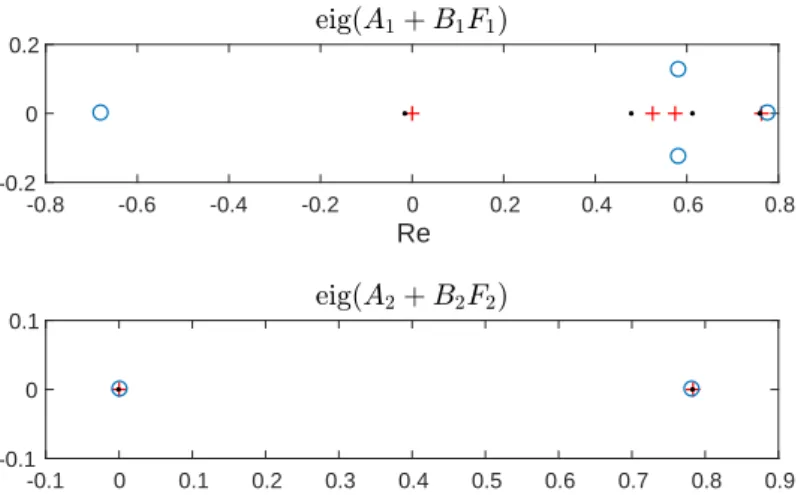
We finally compared the pole locations obtained, as shown in Fig. 2. As can be seen, a better performance was achieved when using the random exciting signal.

3 Summary

In this study, we evaluated different approaches to reducing the effect of measure- ment noise in data-driven pole placement methods for deriving a state space model and pole placement state feedback. Using numerical simulations of a self-balancing

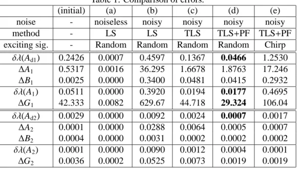
Table 1: Comparison of errors.

(initial) (a) (b) (c) (d) (e)

noise - noiseless noisy noisy noisy noisy

method - LS LS TLS TLS+PF TLS+PF

exciting sig. - Random Random Random Random Chirp δλ(Ad1) 0.2426 0.0007 0.4597 0.1367 0.0466 1.2530

∆A₁ 0.5317 0.0016 36.295 1.6678 1.8763 17.246

∆B1 0.0025 0.0000 0.3400 0.0481 0.0415 0.2932 δλ(A₁) 0.0511 0.0000 0.3920 0.0194 0.0177 0.4695

∆G1 42.333 0.0082 629.67 44.718 29.324 106.04 δλ(A_d2) 0.0029 0.0000 0.0092 0.0024 0.0007 0.0017

∆A₂ 0.0001 0.0000 0.0288 0.0064 0.0005 0.0007

∆B₂ 0.0004 0.0000 0.0031 0.0002 0.0002 0.0002 δλ(A₂) 0.0001 0.0000 0.0090 0.0012 0.0004 0.0001

∆G2 0.0036 0.0002 0.0525 0.0073 0.0019 0.0019

robot, which is a nonlinear system, we demonstrated the important role that pre- filtering can play in reducing the interference caused by noise. Again using numer- ical simulation, we compared the use of two exciting signals: a random signal and a chirp signal. The use of a random exciting signal was found to be more effective with our proposed method. Further developments are needed in the methods used to cope with noise. A method such as that used in [19] may be appropriate for use in practical applications where noise is present, and adaptive control based on real-time updating [16] is a future promising approach.

References

[1] W.M. Wonham, “On pole assignment in multi-input controllable linear sys- tems,” IEEE Transactions on Automatic Control, vol. 12, no. 6, pp. 660- 665, 1967.

[2] J. E. Ackermann, “On the synthesis of linear control systems with specified characteristics,” Automatica, vol. 13, no. 1, pp. 89-94, 1977.

[3] H. Hikita, S. Koyama, and R. Miura, “The redundancy of feedback gain matrix and the derivation of low feedback gain matrix in pole assignment,” The So- ciety of Instrument and Control Engineers, vol. 11, no. 5, pp. 556-560, 1975.

(in Japanese)

[4] S. Yamamoto, Y. Okano, and O. Kaneko, “A data-driven pole placement method simultaneously identifying a state-space model,” Trans. of the Insti- tute of Systems, Control and Information Engineers, vol. 29, no. 4, pp. 275- 284, 2016. (in Japanese)

[5] M. G. Safonov and T.-C. Tsao, “The unfalsified control concept and learning,”

IEEE Transactions on Automatic Control, vol. 42, no. 6, pp. 843-847, 1997.

-0.8 -0.6 -0.4 -0.2 0 0.2 0.4 0.6 0.8 Re

-0.2 0 0.2

Im

-0.1 0 0.1 0.2 0.3 0.4 0.5 0.6 0.7 0.8 0.9

Re -0.1

0 0.1

Im

Figure 2: Comparison of pole locations (‘+’ indicates the desired poles, ‘·’ those obtained by the random exciting signal and ‘◦’ those obtained by the chirp exciting signal).

[6] Y. Matsui, S. Akamatsu, T. Kimura, K. Nakano, and K. Sakurama, “An appli- cation of fictitious reference iterative tuning to state feedback,” The Institute of Electrical Engineers of Japan C, vol. 132, no. 6, pp. 851-859, 2012. (in Japanese)

[7] ZMP Inc., Stabilization and Control of stable running of the Wheeled Inverted Pendulum — Development of Educational Wheeled Inverted Robot e-nuvo WHEEL ver.1.0, http://www.zmp.co.jp/e-nuvo/.

[8] P. E. E. Shwe and S. Yamamoto, “Data-driven method to simultaneously ob- tain a linearized state-space model and pole placement gain,” Proc. of the 3rd Multi-Symposium on Control Systems, 3B3-2, 2016.

[9] H. Kimura, “Pole Assignment by Gain Output Feedback,” IEEE Trans. on Automatic Control, vol. 20, no. 4, pp. 509-516, 1975.

[10] P. E. E. Shwe and S. Yamamoto, “Real-time simultaneously updating a lin- earized state-space model and pole placement gain,” Proc. of SICE 2016, pp. 196-201, 2016.

[11] Z. S. Hou and Z. Wang, “From Model-based Control to Data-driven Control:

Survey, Classification and Perspective,” Information Sciences, vol. 235, pp. 3- 35, 2013.

[12] M. C. Campi, A. Lecchini and S. M. Savaresi, “Virtual Reference Feedback Tuning: A Direct Method for the Design of Feedback Controllers,” Automat- ica, vol. 30,n0. 8, pp. 1337-1346, 2002.

[13] A. Sala and A. Esparza, “Extensions to Virtual Reference Feedback Tun- ing: A Direct Method for the Design of Feedback Controllers,” Automatica, vol. 41,n0. 8, pp. 1473-1476, 2005.

[14] S. Souma, O. Kaneko and T. Fujii, “A New Method of a Controller Parameter Tuning Based on Input-output Data, Fictitious Reference Iterative Tuning,”

In Proceedings of the 2nd IFAC Workshop on Adaptation and Learning in Control and Signal Processing, pp. 789-794, 2004.

[15] Y. Matsui, S. Akamatsu, T. Kimura, K. Nakano and K. Sakurama, “Fictitious Reference Iterative Tuning for State Feedback Control of Inverted Pendulum with Inertia Rotor,” SICE Annual Conference 2011, pp. 1087-1092, 2011.

[16] O. Kaneko, “The Canonical Controller Approach to Data-driven Update of State Feedback Gain,” In Proceedings of the 10th Asian Control Conference 2015 (ASCC 2015), pp. 2980-2985, 2015.

[17] T. Nomura, Y. Kitsuka, H. Suemitsu and T. Matsuo, “Adaptive Backstepping Control for a Two-wheeled Autonomous Robot,” In Proceedings of ICCAS- SICE, pp. 4687-4692, 2009.