Computer-generated holograms for three-dimensional surface objects with shade and texture

(1)

Computer-generated holograms for three-dimensional surface objects with shade and texture

Kyoji Matsushima

Digitally synthetic holograms of surface model objects are investigated for reconstructing three- dimensional objects with shade and texture. The objects in the proposed techniques are composed of planar surfaces, and a property function defined for each surface provides shape and texture. The field emitted from each surface is independently calculated by a method based on rotational transformation of the property function by use of a fast Fourier transform (FFT) and totaled on the hologram. This technique has led to a reduction in computational cost: FFT operation is required only once for calculating a surface. In addition, another technique based on a theoretical model of the brightness of the reconstructed surfaces enables us to shade the surface of a reconstructed object as designed. Optical reconstructions of holograms synthesized by the proposed techniques are demonstrated. © 2005 Optical Society of America

OCIS codes: 090.1760, 090.2870, 090.1970.

1. Introduction

Computer-generated holograms for three- dimensional (3-D) displays, sometimes called digitally synthetic holograms, are desired media for creating 3-D autostereoscopic images of virtual objects. However, the technology suffers from two problems: the necessity for extremely high spatial resolution to fabricate or display the holograms, and long computation times for the creation, especially in full parallax holograms.

For the past decade, techniques using point sources of light have been widely used to calculate object waves.^1,2This point source method is simple in prin- ciple and potentially the most flexible for synthesizing holograms of 3-D objects. However, because it is too time consuming to create full parallax holograms,³ many methods to reduce the computation time, including geometric symmetry,⁴look-up tables,³ difference formulas,⁵recurrence formulas,⁶employing computer-graphics hardware,⁷ and constructing special CPUs,⁸have been attempted.

Point source methods for calculating spherical

waves emitted from point sources are commonly ray oriented. As they trace the ray from a point source to a sampling point on the hologram, the procedure is sometimes referred to as ray tracing.²However, there are also wave-oriented methods to calculate object fields in which fields emitted from objects defined as planar segments^9,10 or 3-D distributions of field strength¹¹are calculated by methods based on wave optics. The major advantage of wave-oriented methods is that they can use a fast Fourier transform (FFT) for numerical calculations. Therefore the computation time is shorter than for point source methods, especially in full parallax holograms. However, the optical reconstruction of accurately rendered 3-D objects such as a shaded cube, as reported for wave- oriented methods, was not discussed in the papers cited above. This is so because of a lack of well-defined procedures to generate object fields for arbitrarily shaped surfaces that are diffusive and sometimes have texture. The technique for shading the reconstructed object according to such design parameters as the position of the illumination light and the ratio of the surrounding light is also important in creating real 3-D images by wave-oriented methods.

In wave-oriented methods, calculating fields are commonly based on coordinate transformation in Fourier space.^10,11 A similar method based on the Rayleigh–Sommerfeld integral has been reported within the context of free-space beam propagation.¹² Recently, the author reported a more precise formu- lation and numerical consideration¹³as an extension

The author ([email protected]) is with the Department of Electrical Engineering and Computer Science, Kansai University, 3-3-35 Yamate-cho, Suita, Osaka 564-8680, Japan.

Received 17 June 2004; revised manuscript received 8 March 2005; accepted 21 March 2005.

0003-6935/05/224607-08$15.00/0

(2)

of an angular spectrum of plane waves¹⁴ in which remapping the angular spectrum plays an important role. The remapping also eases the difficulty of creating object fields in wave-oriented methods.

In this paper two techniques for synthesizing object fields in surface models are presented for creating 3-D images by use of computer-generated holograms.

The first technique, based on the rotational transformation of wave fields presented in Ref. 13 and on remapping of the angular spectrum, provides a method for synthesis of the object fields. This technique makes it possible to create diffusive fields of arbitrarily tilted planar surfaces that have an arbi- trary shape and texture. Furthermore, another technique is also presented for avoiding unexpected changes in brightness of the surfaces of objects. The technique enables us to render surface objects as the designers intended.

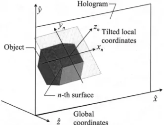
2. Object Model and the Property Function of Surfaces The coordinate systems and geometry used in this study are shown in Fig. 1. Objects consist of planar surfaces that are diffusive and luminous by reflecting virtual illumination. Each surface has its own two local coordinates, called tilt and parallel. The tilted local coordinates defined for the nth planar surface are denoted r_n ⫽ 共x_n,y_n,z_n兲, defined such that the planar surface is laid on the共x_n,y_n, 0兲plane. A complex functionh_n共x_n,y_n兲is defined on the plane to give thenth surface such properties as shape, brightness, diffusiveness, and texture. Thus these complex functions are referred to as the property functions of the surface.

Parallel local coordinates rˆ_n⫽ 共xˆ_n,yˆ_n,zˆ_n兲 are also defined for each surface. They share their origin with the tilted coordinates, but the axes are parallel to those of the global coordinates. In the global coordinates, denotedr⫽共xˆ,yˆ,zˆ兲, the hologram is placed on the共xˆ,yˆ, 0兲plane. All property functions of surfaces are defined in the following form:

h_n(x_n, y_n)⫽a_n(x_n, y_n)⌿(x_n, y_n)p_n(x_n, y_n), (1)

wherea_n共x_n,y_n兲 is a real function that provides amplitudes of the property function to keep the shape and the texture of thenth surface.

If the property function is defined only as the amplitude distribution, the surface yields little diffusiveness, as shown in Fig. 2(a). For example, a_n共x_n,y_n兲 in Fig. 1 is a simple rectangular function; i.e., the amplitude is constant within the rectangular surface.

This situation is similar to the optical diffraction of a plane wave by a rectangular aperture; therefore, if the surface is visible to the naked eye, the light has not been sufficiently diffracted by the aperture. To give surfaces large diffusiveness, the amplitude functions must be multiplied by a given diffusive phase:

⌿(x_n, y_n)⫽exp[ik␾d(x_n, y_n)], (2) where␾d共x_n,y_n兲is a phase that behaves as a numerical diffuser. Random functions are candidates for the diffusive phase, but full random functions are not appropriate to the diffusive phase because the random phases are discontinuous and have a large Fou- rier frequency. Thus the random phases cause speckles in the reconstruction and problems in numerical calculation. In the research reported in this paper, a digital diffuser proposed for Fourier holograms¹⁵is used for phase function␾d共x_n,y_n兲.

If a property function is given by the product of the amplitude function and the diffusive phase, the carrier frequency of the field on the tilted共x_n,y_n, 0兲plane is zero. This forces the surface to emit light perpen- dicularly to the surface, as shown in Fig. 2(b). If the surface is sufficiently diffusive, a portion of the emitted field may reach the hologram, but high diffusiveness results in high computational costs such as the need for a great number of sampling points. There- fore the phase of a plane wave propagating perpen- dicularly to the hologram should be multiplied by the two factors given above. This plane-wave factor causes the field to propagate into the hologram, expressed by

p_n(x_n, y_n)⫽exp[i(k_x,_nx_n⫹k_y,_ny_n)], (3) where k_x,_n and k_y,_n are the x_n and y_n components, respectively, of the wave vector of the plane wave.

The property function given by h_n共x_n,y_n兲 is trans- formed into the complex amplitude hˆ

n共xˆ_n,yˆ_n兲 in the parallel coordinates by the method described in Sec-

Fig. 1. Geometry and definitions of global coordinates and tilted local coordinates defined for a planar surface.

Fig. 2. Fields emitted from surfaces with (a) a constant phase, (b) a diffusive phase, and (c) a diffusive phase multiplied by the phase of a plane wave propagating to a hologram.

4608 APPLIED OPTICS兾Vol. 44, No. 22兾1 August 2005

(3)

tion 5 below. When this transformation is written as hˆ

n(xˆ_n, yˆ_n)⫽᏾␪x␪y␪z{h_n(x_n, y_n)}, (4) fields from all surfaces are superimposed upon the hologram plane as follows:

hˆ(xˆ,yˆ)⫽兺_n ^ᏼ^dⁿ^{h^ˆⁿ^(xˆⁿ^, ^yˆⁿ

(4)

duced in the tilted coordinates:

u⫽u⫺u₀, v⫽v⫺v₀. (13) The spectrum expressed in shifted Fourier space 共u,v兲is written as

H(u, v)⫽H(u⫹u₀, v⫹v₀). (14) The spectrum in the parallel coordinates is obtained by remapping spectrumH共u,v兲onto Fourier space 共uˆ,vˆ兲as follows:

Hˆ(uˆ,vˆ)⬵H(u⫺u₀, v⫺v₀)

⫽H(␣(uˆ,vˆ)⫺u₀, ␤(uˆ,vˆ)⫺v₀), (15) where the sign for nearly equal means that an inter- polation is required.

The Fourier spectrum in the shifted Fourier space is obtained by application of the shift theorem of the Fourier-transform theory to Eq. (14):

H(u, v)⫽Ᏺ{h(x, y)exp[⫺i2␲(u₀x⫹v₀y)]}. (16)

The exponential factor in brackets in Eq. (16) is at- tributed to the carrier frequency observed in the parallel coordinates, whereas factor p共x,y兲 of the property function was introduced to force the emitted field toward the hologram, canceling the carrier frequency in the parallel coordinates. In fact, the exponential factors of Eq. (16) and p共x,y兲 cancel each other out. Equation (16) is rewritten by substitution of Eq. (3) as follows:

H(u, v)⫽Ᏺ{a(x, y)⌿(x, y)exp{i[(k_x⫺2␲u₀)x

⫹(k_y⫺2␲v₀)y]}}, (17) where the subscript n is omitted again. The wave vector of a plane wave propagating along thezˆaxis is expressed by 共0, 0, 2␲兾␭兲 in parallel coordinates.

Thus the plane wave in the tilted coordinates is obtained by coordinates rotation by use of matrix (8) as follows:

k_x⫽2␲a₃兾␭, k_y⫽2␲a₆兾␭. (18) The spectrum of relation (15) is rewritten by substitution of Eqs. (18) and (12):

H(u, v)⫽Ᏺ{a(x, y)⌿(x, y)}. (19) As a result, the factorp共x,y兲is no longer required in the property function if the spectrum is calculated in shifted Fourier space 共u,v兲. Therefore let us rede- fine the property function as

h(x, y)⬅a(x, y)⌿(x, y), (20) and its spectrum as

H(u, v)⬅Ᏺ{h(x, y)}. (21) Consequently, the rotational transformation is summarized as follows: First, one obtains spectrum H共u,v兲 of the property function of Eq. (20) by fast Fourier transformation. The center of the spectrum is placed at the origin in the Fourier space. Next, the spectrum in the parallel coordinates is obtained by remapping spectrumH共u,v兲, expressed by substitut- ing Eq. (12) into relation (15) as follows:

Hˆ(uˆ,vˆ)⬵H(␣(uˆ,vˆ)⫺ ␣(0, 0), ␤(uˆ,vˆ)⫺ ␤(0, 0)).

(22) Finally, the complex amplitudes of the field are obtained in the parallel coordinates by an inverse Fou- rier transformation of Eq. (10).

4. Holograms of a Single Surface with Texture

A. Single Axis Rotation

The hologram of a single planar surface with texture was fabricated for verifying the technique described in Section 5. The planar surface and the hologram are

Fig. 3. Schematic of rotation upon two axes: (a) a plane rotated upon thezˆaxis before thexaxis and (b) resampling areas of the Fourier spectrum at several rotation angles in the rotation scheme.

(5)

sampled at intervals of 2␮m in thexaxis and 4␮m in theyaxis. The planar surface has sampling points of 16,384 ⫻ 4096 and a binary texture. Amplitude distributiona共x,y兲

(6)

change of brightness of a surface is not perceived because there is nothing to compare with the single surface in a piece of hologram. This unexpected and unwanted change of brightness must be resolved if one is to shade the object as intended.

A. Theory of Brightness of Reconstructed Surfaces To compensate for unexpected shading it is necessary to investigate which parameters govern the brightness of the surface in reconstruction. Figure 8 is a theoretical model that predicts the brightness of a surface represented by sampled property function h共x,y兲. Suppose that the amplitude of a property function of a surface is a constant, i.e., that a共x,y兲

⬅a, and suppose thata²provides optical intensity on the surface. In such cases, the radiant flux ⌽ of a small area␦Aon the surface is given by

⌽ ⫽

冕冕

_␦A^|h(x, ^y)|²^dxdy

⬵␦A␴a², (23)

where␴is the surface density of the sampling points.

Assuming that the small area emits light within a diffusion angle in a direction at ␪v to the normal vector, the solid angle corresponding to the diffusion cone is given as⍀ ⫽A兾r², whereA⫽ ␲共rtan␺d兲²is the section of the diffusion cone at a distancerand␺d

is the diffusion angle of light that depends on diffuser function⌿共x,y兲of Eq. (1).

According to photometry, brightness of the surface, observed in a direction at an angle␪v, is given by

L⫽ d⌽兾d⍀

cos␪v␦A. (24)

Assuming that light is diffused almost uniformly, i.e., that d⌽兾dA ⯝ ⌽兾A, the brightness is rewritten by substitution of d⌽⯝ 共⌽兾A兲dA, d⍀ ⫽dA兾r², and relation (23) into Eq. (24) as follows:

L⯝ ␴a²

␲tan²␺dcos␪v

. (25)

As a result, the brightness of the surface depends on the surface density of sampling, the diffusiveness of the diffuser function, and the amplitude of the surface property function. In addition, the brightness of the surface is governed by observation angle␪v. In other words, if several surfaces with the same property function are reconstructed from a hologram, the brightness varies according to the direction of the normal vector of the surface. This phenomenon causes unexpected shading.

Inasmuch as only a simple theoretical model has been discussed so far, relation (25) is only partially appropriate for measuring the brightness of optically reconstructed surfaces of real holograms. The brightness given in relation (25) diverges in the limit

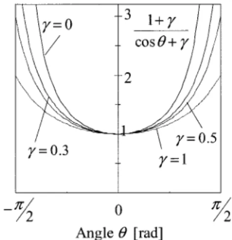
␪v→␲兾2, but an actual hologram cannot produce in- finite brightness for its reconstructed surface. Thus relation (25) is not sufficient to compensate for the brightness. To avoid the divergence of brightness in relation (25), one should introduce angle factor 共1 ⫹ ␥兲兾共cos␪v ⫹ ␥兲 shown in Fig. 9, instead of 1兾cos␪v, a priori. This angle factor is unity in ␪v

⫽ 0 and 1 ⫹ 1兾␥ in ␪v ⫽ ␲兾2. Consequently, the brightness is given as an expression of

L⫽ ␴a²

␲tan²␸d

(1⫹ ␥)

(cos␪v⫹ ␥), (26) where␥is a parameter that plays a role in preventing the divergence of brightness and in preventing over- compensation. Because ␥ is dependent on actual methods for fabricating holograms, such as encoding the field or the property of recording materials, it should be determined experimentally.

B. Compensation for Brightness and Shading Objects The amplitude of a property function that recon- structs a surface in a given brightnessLis obtained by solution of Eq. (26) foraas follows:

a⫽

冋

^L^␲^tan^␴ ²^␸^d ^(cos⁽¹^␪^{⫹ ␥}^v^{⫹ ␥}⁾ ⁾

册

^1兾2^. ⁽²⁷⁾

Fig. 8. Model of brightness of a planar surface expressed by a property function sampled at an equidistant grid.

Fig. 9. Curves of the angle factor for several values of␥.

(7)

However, angle ␪v is unknown in synthesizing the object field, and therefore it seems impossible to compensate for the change of brightness. But holograms are observed in a direction along thezˆaxis, i.e., per- pendicular to the hologram, because the hologram is usually observed at a distance of more than several tens of centimeters. Hence it is possible to approxi- mate␪vby an angle␪nformed between the nth sur- face and the hologram. Objects are shaded by a method based on Lambert’s law and the diffused re- flection model. The brightness of the nth surface, of which the normal vector forms angle^␪

nwith the vector of illumination, is given by

L_n⫽L₀(cos␪^

n⫹l_e), (28)

where l_eis the ratio of the surrounding light to the illumination and L₀ is brightness in ^␪

n ⫽ 0 and l_e

⫽0. By substitution ofL_nof Eq. (28) intoLof Eq. (27) amplitudea_nof thenth surface is given as follows:

a_n⫽a₀

冋

^(cos^␪^{^}ⁿ^⫹¹^l^e^{⫹ ␥}^)(cos^␪ⁿ^{⫹ ␥}⁾

册

^1兾2^, ⁽²⁹⁾

a₀⬅

冋

^L⁰^␲^tan^␴ ²^␸^d

册

^1兾2^. ⁽³⁰⁾

Here, observation angle␪vis replaced by the angle of the normal vector,␪n.

6. Optical Reconstruction of Three-Dimensional Objects

First, I fabricated several holograms of the same hexagonal prism with which to determine the value of parameter␥. Figure 10 shows the optical reconstruction of three holograms. The reconstructed image of the hologram without compensation for brightness is shown in Fig. 10(a). The left-hand surface of the hexagonal prism, which has the largest angle␪n, is the brightest of the object surfaces. As shown in Fig.

10(b), the hologram with compensation in ␥ ⫽ 0 is contrasted to that in Fig. 10(a). Here, remember that compensation in␥ ⫽0 leads to unlimited compensation. Therefore the surface that forms a large angle with the hologram is dark as a result of overcompen- sation. Figure 10(c) is also applicable to a hexagonal prism whose brightness is compensated for by

␥ ⫽0.5. Differences of brightness disappear by proper compensation for brightness, which dissolves borders between surfaces.

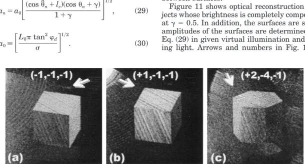
Figure 11 shows optical reconstruction of 3-D objects whose brightness is completely compensated for at␥ ⫽0.5. In addition, the surfaces are shaded; the amplitudes of the surfaces are determined by use of Eq. (29) in given virtual illumination and surrounding light. Arrows and numbers in Fig. 11 indicate

Fig. 10. Optical reconstructions of unshaded hexagonal prisms (a) without brightness compensation and (b), (c) with compensation in

␥ ⫽0, 0.5, respectively.

Fig. 11. Optical reconstructions of 3-D objects shaded with illumination light. Cubes are illuminated from the upper right in (a)le⫽0 and from the upper left in (b)le⫽0.7; a hexagonal prism共le⫽0.5兲is shown in (c). Brightnesses of objects are all compensated for at␥ ⫽0.5. Arrows and numbers in parentheses define the illumination vector in global coordinates.

(8)

illumination vectors in global coordinates. As ex- pected from the vectors, object surfaces are shaded in the reconstructions.

7. Discussion

The computation time in the proposed techniques is given by rotational transformation of the surfaces of the object. According to Ref. 13, the computation time of rotational transformation is dominated by FFTs, and FFT operation must be executed twice to rotate a planar surface. However, most of the inverse FFTs of Eq. (10) can be omitted from calculating the total field; just an inverse FFT operation is necessary to create a hologram because the translational propagation of the fieldᏼd兵其can be carried out in Fourier space. In the synthesis of holograms described in pre- vious sections, the method of the angular spectrum of plane waves¹⁴is used for the operation of the propagation. Therefore the total field of Eq. (5) on the hologram is expressed by

hˆ(xˆ,yˆ)⫽Ᏺ^⫺1兵^兺ⁿ ^H^ˆⁿ^(u^ˆⁿ^, ^vˆⁿ^)exp[i2^␲^w^ˆ^(u^ˆ^n,^vˆⁿ^)dⁿ^]其^,

(31) whered_nis the distance between the共xˆ_n,yˆ_n, 0兲plane of the parallel coordinates and the hologram. Thus the number of times a FFT is executed isN⫹ 1, to calculate the total field of an object composed of N pieces of planar surface. As a result, one FFT兾surface is approximately estimated as the computational cost in the proposed techniques.

8. Conclusion

Full parallax computer-generated holograms of three-dimensional surface objects were synthesized by use of a wave-optical method. In this method, an object is composed of some planar surfaces, and a complex function defined for each surface retains such properties as shape, texture, and brightness.

The fields emitted from the tilted surfaces are calculated by use of the rotational transformation of the property function and totaled on the hologram.

When surfaces build an object, the change of brightness that depends on the angle of view causes unexpected shading of the surface. A theoretical model with which to predict the brightness of the reconstructed surface and prevent unexpected shading has been proposed. This technique allows the object to be shaded as one intends. Finally, optical reconstructions of holograms synthesized by use of the proposed techniques have been demonstrated to verify the validity of the methods.

This study is partly supported by the Kansai Uni- versity High Technology Research Center and in part by Kansai University research grants, including a grant-in-aid for encouragement of scientists, in 2003.

References

1. J. P. Waters, “Holographic image synthesis utilizing theoretical methods,” Appl. Phys. Lett.9,405– 407 (1966).

2. A. D. Stein, Z. Wang, and J. J. S. Leigh, “Computer-generated holograms: a simplified ray-tracing approach,” Comput. Phys.

6,389 –392 (1992).

3. M. Lucente, “Interactive computation of holograms using a look-up table,” J. Electron. Imag.2,28 –34 (1993).

4. J. L. Juárez-Pérez, A. Olivares-Pérez, and R. Berriel-Valdos,

“Nonredundant calculation for creating digital Fresnel holograms,” Appl. Opt.36,7437–7443 (1997).

5. H. Yoshikawa, S. Iwase, and T. Oneda, “Fast computation of Fresnel holograms employing difference,” inPractical Holog- raphy XIV and Holographic Materials VI, S. A. Benton, S. H.

Stevenson, and J. T. Trout, eds., Proc. SPIE 3956, 48 –55 (2000).

6. K. Matsushima and M. Takai, “Recurrence formulas for fast creation of synthetic three-dimensional holograms,” Appl. Opt.

39,6587– 6594 (2000).

7. A. Ritter, J. Böttger, O. Deussen, M. König, and T. Strothotte,

“Hardware-based rendering of full-parallax synthetic holograms,” Appl. Opt.38,1364 –1369 (1999).

8. T. Ito, H. Eldeib, K. Yoshida, S. Takahashi, T. Yabe, and T.

Kunugi, “Special purpose computer for holography HORN-2,”

Comput. Phys. Commun.93,13–20 (1996).

9. D. Leseberg and C. Frère, “Computer-generated holograms of 3-D objects composed of tilted planar segments,” Appl. Opt.27, 3020 –3024 (1988).

10. T. Tommasi and B. Bianco, “Computer-generated holograms of tilted planes by a spatial frequency approach,” J. Opt. Soc. Am.

A10,299 –305 (1993).

11. D. Leseberg, “Computer-generated three-dimensional image holograms,” Appl. Opt.31,223–229 (1992).

12. N. Delen and B. Hooker, “Free-space beam propagation between arbitrarily oriented planes based on full diffraction theory: a fast Fourier transform approach,” J. Opt. Soc. Am. A15, 857– 867 (1998).

13. K. Matsushima, H. Schimmel, and F. Wyrowski, “Fast calculation method for optical diffraction on tilted planes by use of the angular spectrum of plane waves,” J. Opt. Soc. Am. A20, 1755–1762 (2003).

14. J. W. Goodman, Introduction to Fourier Optics, 2nd ed.

(McGraw-Hill, 1996), Chap. 3.10.

15. R. Bräuer, F. Wyrowski, and O. Bryngdahl, “Diffusers in digital holography,” J. Opt. Soc. Am. A8,572–578 (1991).

16. K. Matsushima and A. Kondoh, “Wave optical algorithm for creating digitally synthetic holograms of three-dimensional surface objects,” in Practical Holography XVII and Holo- graphic Materials IX, T. H. Jeong and S. H. Stevenson, eds., Proc. SPIE5005,190 –197 (2003).

17. K. Matsushima and A. Joko, “A high-resolution printer for fabricating computer-generated display holograms (in Japa- nese),” J. Inst. Image Inf. Television Eng. 56, 1989 –1994 (2002).