SAR Image Analysis and Target Detection Utilizing Polarimetric Information

SAR Image Analysis and Target Detection Utilizing Polarimetric Information

DISSERTATION

submitted in partial satisfaction of the requirements for the degree of

DOCTOR OF PHILOSOPHY

National Defense Academy

Graduate School of Science and Engineering

Electronics and Information Engineering

Concentration in Computer, Intelligent and Media Systems

Mitsunobu Sugimoto

March 2013

Table of Contents

Page

Table of Contents ii

List of Figures iv

List of Tables viii

List of Symbols and Abbreviations ix

Acknowledgments xiv

Abstract of the Dissertation xvi

1 Introduction 1

1.1 Synthetic Aperture Radar . . . 1

1.2 Selected Spaceborne and Airborne SAR . . . 4

1.3 Other Recent Trends in SAR . . . 8

1.4 Purpose of This Study . . . 10

1.5 Outline of the Thesis . . . 11

2 SAR Fundamentals 13 2.1 SAR System Parameters . . . 14

2.1.1 Geometry of SAR System . . . 14

2.1.2 Signal Parameters . . . 15

2.2 Image Formation in Range Direction . . . 16

2.2.1 Image Formation with Rectangular Pulses . . . 17

2.2.2 Image Formation with the Pulse Compression Technique . . . 18

2.3 Image Formation in Azimuth Direction . . . 26

2.3.1 Image Formation with Real Aperture Radar . . . 26

2.3.2 Image Formation with Aperture Synthesis . . . 30

3 SAR Polarimetric Analysis 40 3.1 Polarization State of Electromagnetic Waves . . . 41

3.2 Matrix Representation of PolSAR Data . . . 44

3.3 Model-based Decomposition Analysis . . . 48

3.4 Eigenvalue Decomposition Analysis . . . 50

4 4-CSPD Algorithm with Rotation of Covariance Matrix 56

4.1 Overview . . . 57

4.2 Rotation of Covariance Matrix . . . 59

4.3 4-CSPD Algorithm Using Rotated Covariance Matrix . . . 62

4.4 Experimental Results and Discussions . . . 65

5 Comparison between Eigenvalue Analyses of Different Polarization 71 5.1 Introduction . . . 72

5.2 Methodology . . . 73

5.3 Polarimetric SAR Data . . . 75

5.4 Experimental Results and Discussions . . . 75

6 Marine Target Detection Using the Model-Based Decomposition 82 6.1 Introduction . . . 83

6.2 Methodology . . . 84

6.3 PolSAR Data and Ground Truth . . . 86

6.4 Experimental results and Discussions . . . 89

7 Comprehensive Comparison of Different Polarimetric Methods 96 7.1 Introduction . . . 97

7.2 Interaction between Laver Cultivation Area and SAR Microwaves . . 98

7.3 Experimental results and Discussions . . . 100

8 Conclusions 111

Bibliography 115

List of Figures

Page 1.1 Illustrating the three active microwave instruments on board of SEASAT.

The radar scatterometer consisting of two pairs of three rod antennas was used to measure ocean winds, and the parabola antenna point- ing at nadir was the radar altimeter to measure ocean surface height.

The SAR antenna was 10.7m in the along-track direction and 2.2m in the cross-track direction with the off-nadir angle of 23^◦. (Courtesy of

NASA/JPL) . . . 2

1.2 Outline of the thesis . . . 12

2.1 Illustration of SAR geometry. . . 15

2.2 Pulses and observation window of spaceborne SAR. f_p is pulse rep- etition frequency, t_p is pulse repetition time and the inverse number of f_p, and τ_w is the time duration of the observation window. The observation window is for the first transmitted pulse. . . 16

2.3 Illustrating range imaging process and resolution of a conventional radar with rectangular pulses. . . 18

2.4 Illustrating (a) the real component of the phase of a FM pulse and (b) instantaneous frequency withω_c= 0. . . 20

2.5 Change of coordinate origin in slant-range time. (a) Origin at the antenna. (b) Origin at the ground. . . 23

2.6 Intensity point spread function in range direction. . . 24

2.7 Illustrating azimuth resolution of a conventional radar. . . 28

2.8 (a) Beam pattern in azimuth direction. (b) Resolution: in the case of sinc function beam pattern. . . 29

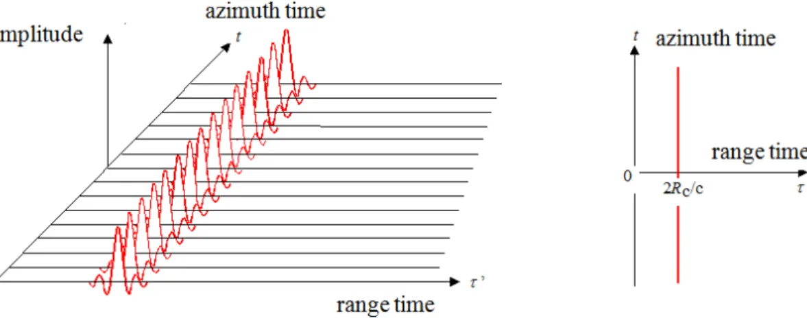
2.9 Illustration of a geometry of a point scatterer and the platform at different azimuth times. . . 30

2.10 Aligned received pulses. . . 32

2.11 Top view of the re-arranged 2-D signal. . . 33

2.12 A received 2-D signal after the range compression. . . 34

2.13 A received 2-D signal after the range migration compensation. . . 35

3.1 Electric field of linear polarization. . . 41

3.2 Electric field of circular polarization. . . 42

3.3 Polarization ellipse. . . 43

3.4 Varying polarization state by different ellipticity and tilt angles. Power is for the polarization signature. . . 44 3.5 Feasible region in H−α¯ plane for random media scattering problems

[28]. . . 53 4.1 4-CSPD algorithm using rotation of covariance matrix (the structure

of entire flowchart mainly comes from [46]). . . 63 4.2 ALOS-PALSAR decomposition images of Tokyo Bay, Japan. The cen-

tral coordinate of each image is approximately at (139^◦52’E, 35^◦20’N).

The upper row (a,b): 4-CSPD (the helix component were excluded).

The lower row (c,d): 4-CSPD with rotation. The left column (a,c) shows results from coherency matrix and the right column (b,d) shows results from covariance matrix. The red, green, and blue colors rep- resent the double-bounce, volume, and surface scattering components respectively. Areas A, B, and C are mostly composed of urban, moun- tainous, and sea areas respectively. Area D is an area which shows remarkable change after rotation. . . 66 4.3 Optical photograph of the image corresponding to the area in Figure

4.2. The central coordinate of the image is approximately at (139^◦52’E, 35^◦20’N). . . 68 4.4 Rotation Angle distribution of the selected areas in Figure 4.2. Hori-

zontal axis is rotation angle and vertical axis is frequency. (a) Area A.

(b) Area B. (c) Area C. (d) Area D. . . 69 4.5 Tokyo Bay Aqua-Line (Highway) near the area of Figure 4.2. The cen-

tral coordinate of each image is approximately at (139^◦53’E, 35^◦26’N).

(a) 4-CSPD image without rotation. (b) 4-CSPD image with rotation.

(c) Difference of the P_d component between the left and the middle image. . . 70 4.6 Tokyo Bay Aqua-Line (Highway) near the area of Figure 4.2. (a) Rota-

tion angle image. The central coordinate of the image is approximately at (139^◦53’E, 35^◦27’N). (b) Rotation angle distribution of the left im- age. The peak around 30 degree represents the highway bridge. . . . 70 5.1 The original ALOS-PALSAR quad-polarization amplitude images ac-

quired on 24 November 2008 over the Tokyo Bay, Japan. (a) HH polarization image. (b) VV polarization image. (c) HV polarization image. . . 78 5.2 Comparison between quad- (upper row), HH/VV dual- (middle row),

and HH/HV dual- (lower row) entropy/alpha decomposition. (a) Quad entropy image. (b) Quad alpha angle image. (c) HH/VV dual entropy image. (d) HH/VV dual alpha image. (e) HH/HV dual entropy image.

(f) HH/HV dual alpha image. . . 79

5.3 Enlarged images of selected areas from Figure 5.2. From left to right column, sea, vegetation, and urban areas are shown. (a)-(c) Quad entropy. (d)-(f) HH/VV dual entropy. (g)-(i) HH/HV dual entropy.

(j)-(l) Quad alpha angle. (m)-(o) HH/VV dual alpha angle. (p)-(r) HH/HV dual alpha angle. . . 80 5.4 Entropy/alpha plots of selected areas from quad- (upper row), HH/VV

dual- (middle row), and HH/HV dual- (lower row) eigenvalue analyses.

From left to right column, sea, vegetation, and urban areas are shown.

(a)-(c) Quad entropy/alpha plot. (d)-(f) HH/VV dual entropy/alpha plot. (g)-(i) HH/HV dual entropy/alpha plot. . . 81 6.1 Scattering from ships. . . 84 6.2 Flowchart of detection process. . . 86 6.3 A Google Map image of the area around Portsmouth. The central co-

ordinate of the image is approximately at 50^◦45’N, 1^◦04’W. The white rectangle at the center of the image represents the test site analyzed in this study. Imagery c⃝2012 TerraMetrics. Map data c⃝2012 Google (accessed November 6, 2012). . . 87 6.4 The ALOS-PALSAR quad-polarization amplitude images and the de-

composed image. The image centre is approximately at 50^◦46’N, 1^◦04’W and the image size is approximately 5 km in both azimuth and range directions. (a) HH image. (b) VV image. (c) HV image. (d) De- composed image of the test site (red: double-bounce scattering, green:

volume scattering, blue: surface scattering). The white rectangle is an area chosen as the homogeneous background area. . . 88 6.5 Nautical map as reference data. ⃝cPortsmouth Port 2011 (accessed

November 5, 2012). . . 90 6.6 (a)T P−P_s image. (b) Statistical intensity distribution of background

area marked as rectangles in (a) and candidate PDFs. . . 91 6.7 (a) Optimized P_d image. (b) Statistical intensity distribution of back-

ground area marked as rectangles in (a) and candidate PDFs. . . 91 6.8 Receiver operating characteristic (ROC) curves. . . 92 6.9 Detection result by TP −P_s (solid circles: detected targets, dashed

circles: missed targets). . . 93 6.10 Detection result by optimizedP_d(solid circles: detected targets, dashed

circles: missed targets) . . . 93

6.11 Ship detection using fully polarimetric ALOS-PALSAR data around Tokyo bay on 9 October, 2008. The image center is at approximately 35^◦17’N, 139^◦44’E, and the image size is approximately 10 km in range and 7 km in azimuth directions. Solid circles: visible/detected tar- gets. Dashed circles: invisible/missed targets. Rectangles: two sea forts (top) and an island (left). (a) Decomposed image of the test site obtained using the 4-CSPD algorithm (red: double-bounce scatter- ing, green: volume scattering, blue: surface scattering). (b) Detection result obtained by excluding the surface scattering component. (c) Detection result obtained using the optimized Pd. . . 95 7.1 Photograph of a part of the Futtsu Horn test area in Tokyo Bay, Japan

taken on 5th of February 2011. . . 99 7.2 The ALOS-PALSAR quad-polarization amplitude images acquired on

24 November 2008 over Tokyo Bay, Japan. (a) HH polarization image.

(b) VV polarization image. (c) HV polarization image. . . 100 7.3 Comparison of image contrast between laver cultivation area and back-

ground area using methods with HH and VV dual-polarization combi- nation from ALOS-PALSAR data. . . 104 7.4 Comparison of image contrast between laver cultivation area and back-

ground area using methods with quad-polarization data from ALOS- PALSAR. . . 105 7.5 TerraSAR-X amplitude images of Futtsu Horn laver cultivation area

in Tokyo Bay, Japan. The data were acquired on October 20, 2011 (upper row (a) and (b)) and December 26, 2008 (lower row (c) and (d)). (a)(c): HH amplitude image. (b)(d): VV amplitude image. . . . 106 7.6 Comparison of image contrast between laver cultivation area and back-

ground using TerraSAR-X HH/VV dual-polarization data in 2011. The values next to each caption are mean contrasts. (a) HH+VV image:

0.001. (b) HH-VV image: 0.327. (c) Entropy image: 0.253. (d) Scat- tering angle image: 0.348. (e) HH/VV coherence image: 0.674. (f) Phase difference image: 0.226. . . 109 7.7 Comparison of image contrast between laver cultivation area and back-

ground using TerraSAR-X HH/VV dual-polarization data in 2008. The values next to each caption are mean contrasts. (a) HH+VV image:

0.254. (b) HH-VV image: 0.244. (c) Entropy image: 0.465. (d) Scat- tering angle image: 0.008. (e) HH/VV coherence image: 0.031. (f) Phase difference image: 0.008. . . 110

List of Tables

Page 1.1 Selected fields of SAR application examples. Note that not all appli-

cations are in practical use; many applications are still at developing stages [3]. . . 2 1.2 Parameters of selected spaceborne SARs. “Pol.” means the available

combination of polarization states, “Res.” indicates the finest available spatial resolutions in azimuth/range directions, “Weight” is in kg, and

“Alt.” is the average orbit altitude in km. The parentheses next to sensor name are the number of identical satellites. . . 5 1.3 Common frequency bands for radar systems. . . 8 1.4 Parameters of selected airborne SARs. “Res.” indicates the maximum

achievable spatial resolutions in azimuth/range directions. Most of the listed airborne SARs operate in quad- (quadrature) polarization with interferometric modes. UAV next to sensor name stands for Unmanned Aerial Vehicle. . . 9 4.1 Relative contribution to total power of Tokyo Bay area before and after

rotation. . . 67 5.1 Quantitative evaluation of differences between quad- and HH/VV dual-

analysis or between quad- and HH/HV dual-eigenvalue analysis. The values without parenthesis are results from quad- and HH/VV dual- eigenvalue analysis and the values in parenthesis are results from quad- and HH/HV dual-eigenvalue analysis. . . 77 7.1 Image contrast comparisons between the cultivation area and the back-

ground area. . . 103 7.2 Details of TerraSAR-X data used in this study. The incidence angles

are at the center of the test site in Figure 7.5. . . 107 7.3 Image contrast between laver cultivation area and background area

using TerraSAR-X HH/VV dual-polarization data (Figure 7.5, 7.6 and 7.7). . . 108

List of Symbols and Abbreviations

A Anisotropy

B Bandwidth

B_A Doppler Bandwidth

B_D Effective Doppler Bandwidth B_R Chirp Bandwidth

C Covariance Matrix

C(θ) Rotated Covariance Matrix

D_A Antenna Length

E Amplitude of Electric Field E₀ Amplitude of Received Signal E₀^′ Amplitude of Transmitted Signal

E_0y′, E_0z′ Minor and Major Semi-Axes of the Ellipse E_r Reference Signal

ER PSF in Range Direction E_s,E_s^′ Received Signal

E_t Transmitted Signal E Electric Field Vector

E_y, E_z y-Component and z-Component ofE H Polarimetric Scattering Entropy L₀ Beam Width in Azimuth Direction

P Probability

P_s, P_d, P_v, P_c Power of Surface, Double-Bounce, Volume, and Helix Scattering R Slant-Range Variable (Distance)

R₀ Shortest Slant-Range Distance between Platform and Target R_c Arbitrary Slant-Range Distance

S Sinclair Scattering Matrix

T Coherence Matrix

T P Total Power

T₀ Illuminating Time

T_A Integration Time (Aperture Synthesis Time)

U Unitary Matrix

U_θ Unitary Rotation Matrix

V Platform Speed

W_A Absolute Amplitude Value in Azimuth Direction Y Azimuth Spatial Variable (Distance)

Y Ground-Range Spatial Variable (Distance)

a, b Unknown Parameters in Model-Based Decompositions

c Speed of Light

f Instantaneous Frequency f₀ Radar Frequency

f_DC Doppler Center Frequency

f_a Doppler Instantaneous Frequency f_p Pulse Repetition Frequency

fs, fd, fv Surface, Double-Bounce and Volume Scattering Contributions h Altitude of Platform

k Wavenumber Equal to 2π/λ k Scattering Vector

p Azimuth Space Variable (Platform Position)

r_j Slant-Range Distance between Antenna and Scatterer at j th Pulse r(t) Slant-Range Distance between Antenna and Scatterer at Azimuth Time

t

t Time Variable in Azimuth Direction t^′ Time Variable in Azimuth Image Plane t_p Pulse Repetition Time

t_j j th Pulse Transmission Time

u Eigenvector

v_E Slant-Range Velocity Component Associated with the Earth s Rotation x, y, z Cartesian Coordinate System

∆X Azimuth Resolution

∆Y Ground-Range Resolution

∆τR Size of the Resolution Cell (Time)

∆θ_A Beam Spread Angle in Azimuth Direction Ψ_HV HV Linear Polarization Basis

Ψ_P Pauli Basis

α Frequency Modulation Rate

¯

α Alpha Angle

β Doppler Constant

β¯ Beta Angle

θ Rotation Angle

θ_i Incidence Angle θ0 Off-nadir Angle

λ Wavelength

λ₁, λ₂, λ₃ Eigenvalues of Coherence Matrix τ Time Variable in Range Direction

τ^′ Time Variable in Range Image Plane

τ_R Time Variable in Range Direction (Origin at the Ground) τ_p Transmitted Pulse Duration

τ_w Time Duration of Observation Window ϕ Phase of Complex Amplitude

φ Tilt Angle

χ Ellipticity Angle ψ Phase of Chirp Pulse ω_c Centre Radian Frequency

⟨·⟩ Ensemble Average

4-CSPD Four-Component Scattering Power Decomposition CFAR Constant False Alarm Rate

DEM Digital Elevation Model DSM Digital Surface Model EM Electromagnetic FAR False Alarm Rate FM Frequency Modulation

GIS Geographic Information System HH horizontal transmission and reception

HV horizontal transmission and vertical reception IRF Impulse Response Function

MCLM Multiple-Component Scattering Model PDF Probability Density Function

PRF Pulse Repetition Frequency PRT Pulse Repetition Time PSF Point Spread Function RAR Real Aperture Radar

RCS Radar Cross Section RMSE Root-Mean-Square-Error

ROC Receiver Operating Characteristic SAR Synthetic Aperture Radar

TBP Time Bandwidth Product

VH Vertical transmission and horizontal reception VV Vertical transmission and reception

Acknowledgments

My gratitude goes first to my advisor Professor Yasuhiro Nakamura who has inspired me with his profound and insightful advice since I joined in the software engineering lab at National Defense Academy.

I would like to express my sincere gratitude to Professor Kazuo Ouchi, for his invalu- able support, patience, and supervision throughout my research work. He is the man who introduced me into the exciting world of synthetic aperture radar. Without his consistent guidance and encouragement this thesis would not have been possible. He has always been willing to help and my three years of study went smoothly and was truly rewarding for me. All of what he has taught me during the doctoral course will be an invaluable asset for the rest of my life.

Thanks also go to my thesis committee members, Professor Hisashi Morishita and Professor Hajime Fukuchi, for their invaluable advice and comments to improve my thesis.

I thank Lecturer Munetoshi Iwakiri and my fellow lab mates. My research work has been a cozy and memorable experience for me because of each one of you.

My thank also goes to many friends who assisted, advised, and encouraged me during my research work.

I would like to thank the Japan Ground Self-Defense Force, and especially its people

for all the financial, logistic, and mental supports they have given to me during my graduate studies.

Finally, I am truly grateful to Keiko, Kaina, and Mina for all their immeasurable love and support. They all are source of my energy and motivation.

Abstract of the Dissertation

SAR Image Analysis and Target Detection Utilizing Polarimetric Information

By

Mitsunobu Sugimoto

Doctor of Philosophy in Electronics and Information Engineering Concentration in Computer, Intelligent and Media Systems

Graduate School of Science and Engineering, March 2013

合成開口レーダ（SAR）のデータ解析においてポラリメトリ（偏波解析）は，異な る偏波コンビネーションの送受信レーダ情報を用いて観測対象の特性を計測する技術 である。近年の

の多偏波化のトレンドに伴い現在注目が高まっているが，ポラ リメトリを用いた解析手法間の比較，もしくはグラウンドトゥルースデータとの定量 的比較は十分に行われていないのが実情である。本論文は

ポラリメトリック情 報を活用した画像解析の手法とそのターゲット検出への応用についての研究を行い，

成果をまとめたものである。大きく分けると，第

章が本研究の背景についての 系統ごとのまとめ，第

章が本研究における画像解析手法に関する研究成果，第

章が本研究における観測ターゲット検出に関する研究成果となっている。

第

章では，

以来の衛星及び航空機搭載

とその関連技術につい

ての歴史を簡潔に紹介するとともに，本研究の目的と本論文の構成を明らかにする。

SAR

の近年の傾向としては，高解像度化（衛星搭載

においては数

載

においては数十

・多偏波化・プラットフォーム軽量化・衛星搭載

の

回帰日数の短縮等が挙げられる。ポラリメトリの他に注目を集めている

の技術

の一つとしてインタフェロメトリがある。インタフェロメトリは，同一の観測対象地 域を，SAR プラットフォーム軌道上の微妙に異なる位置から観測した

セットの複素 画像を干渉させ，位相情報の差を解析することにより地表高度や地殻変化を高精度で 計測する技術である。インタフェロメトリは多偏波情報を必要としないため，ポラリ メトリと比較して研究の歴史が長く，実用段階に達している

データ利用技術の 一つである。

第

章では，SAR の画像生成プロセスについて説明する。SAR は高解像度の二次 元レーダ画像を生成する。アジマス方向と呼ばれる

プラットフォームの進行方 向の画像生成においては，プラットフォーム搭載のアンテナとプラットフォームの移 動によるドップラー効果を活用することにより仮想的に非常に大きな開口を合成する ことで高解像度を達成する。SAR の名称の由来はここから来ている。レンジ方向と 呼ばれるアジマス方向に直交する方向の画像生成においては，送信信号そのものを ドップラー信号として送信し，かつパルス圧縮技術を用いることにより高解像度を達 成する。

第

章では，SAR ポラリメトリについて説明する。ポラリメトリは，観測ターゲッ トに関するより詳細な情報を含んだ多偏波

データを用いる解析技術である。そ のため，多偏波データを用いることで，従来の単偏波データを用いた解析手法に比 べ観測ターゲットのより詳細な分類が可能になると期待されている。現在のところ，

広く用いられている偏波解析手法は二つあり，一つが

成分分解を代表とするモデル ベース分解法，もう一つが固有値解析法である。

第

章では，共分散行列を用いた回転

成分分解アルゴリズムについて述べる。4

成分分解はモデルベース分解法の一つであるが，近年，偏波行列を回転させることに

より都市域の分類精度を向上させる改善が提案された。本章では，上記のアルゴリズ

ムを用いて得られた結果がコヒーレンシ行列の回転アルゴリズムを用いて得られた結

果と一致することを実データを用いて実験的に示す。理論的には，これら二つの行列

散行列を直接回転させ成分分解した場合のアルゴリズムに対する実データを用いた検 証は行われていなかった。

第

章では，2 偏波のみを用いた固有値解析法の結果を，4 偏波すべてを用いた固 有値解析法と比較した。結果として，HH/VV の２偏波から得られる結果はエントロ ピー・α角ともに４偏波から得られる結果と高い相関性を持つことが明らかになった。

また，HH/HV の２偏波からは，α角の有用な情報を得ることは困難であるが，エン トロピーの値は

ほどではないものの４偏波と高い相関性を持つことが明らか になった。

第

章では，モデルベース分解法の結果を応用した海上人工物の検出手法について 述べる。本来，モデルベース分解法は陸域の様々な特徴を持った観測対象の分類を目 的に提案されたものであったため，海面がほとんどを占める海洋での応用は注目され てこなかった。しかしながら，海面上の人工物というのは海面そのものと比較して明 確に異なった散乱特性を持つため，これを利用して海上人工物の検出が可能である。

ここでは，二つのアプローチを提案する。一つがモデルベース分解法の結果を帯域除 去フィルタとして用いる手法，もう一つが第

章のアルゴリズムを用いる手法である。

第

章では，第

章，5 章の手法を含めた

ポラリメトリにおける代表的な手法

を横断的に用い，海上の海苔養殖場の検出実用度についてコントラストを基準として

包括的に評価した。これにより，利用できる偏波情報の違いに応じた検出結果の良否

が相対的・定量的に明らかにされた。

Chapter 1

Introduction

1.1 Synthetic Aperture Radar

Synthetic Aperture Radar (SAR) is an imaging radar, which can produce high- resolution radar images of earth’s surface from airborne and spaceborne platforms [1, 2]. Since SAR is an active sensor and uses the microwave band in the broad radio spectrum, it has a day-and-night imaging capability, and an ability of penetrating cloud cover, and to some extent, rain. Because of these characteristics, SAR has been used in various fields of geoscience, engineering and military as listed in Table 1.1.

The dawn of the present SAR technology can be placed at the launch of the marine observation satellite SEASAT (Figure 1.1) by NASA in 1978. SEASAT was the first spaceborne SAR designed for the purpose of earth observation. SEASAT-SAR operated at L-band (frequency: 1.275GHz, wavelength: 23.5cm), and the spatial resolution was 6.25m (full-look) and 25m in the along-track and cross-track directions respectively. Despite its short life time of 106 days, SEASAT-SAR produced fine radar images of earth’s surface, and lead to the world-wide extensive research on developing

Table 1.1: Selected fields of SAR application examples. Note that not all applications are in practical use; many applications are still at developing stages [3].

Fields Objects

Geology topography, DEM & DSM production, diastrophism, faults, GIS, lithology, soil structure, underground resources

Agriculture crop classification, plantation acreage, growth, harvest, soil moisture

Forestry tree biomass, height, species, plantation & deforestation, wildfire monitoring Hydrology soil moisture, wetland, drainage pattern, river flow, water resources in desert

water equivalent snow & ice water cycle

Urban urban structure & density, change detection, subsidence, traffic monitoring urbanization, skyscraper height estimation

Disaster prediction, lifeline search, monitoring of damage & recovery, tsunami & high tide, landslide & subsidence by earthquake, volcano & groundwater extraction

Oceanography ocean waves, internal waves, wind, ship detection, identification & navigation, ocean currents, front, circulation, oil slick, offshore oil field, bottom topography Cryosphere classification, distribution & changes of ice & snow on land, sea & lake, ice age,

equivalent water, glacier flow, iceberg tracking, ship navigation in sea ice Archeology exploration of aboveground and underground remains, survey, management Military reconnaissance, search, identification & change detection of targets & traces,

damage assessment

Figure 1.1: Illustrating the three active microwave instruments on board of SEASAT.

The radar scatterometer consisting of two pairs of three rod antennas was used to measure ocean winds, and the parabola antenna pointing at nadir was the radar altimeter to measure ocean surface height. The SAR antenna was 10.7m in the along-track direction and 2.2m in the cross-track direction with the off-nadir angle of 23^◦. (Courtesy of NASA/JPL)

the techniques to utilize the wealth of potential information contained in the SAR data [4]. At the time of SEASAT, intensity or amplitude images were of main interest, and little consideration was given to preserving the phase in SAR processors. Of course, amplitude data are the basis of SAR image analysis, and contain much information on scattering media. Utilization of amplitude data is still a subject of current research.

The additional potential information suggested by SEASAT-SAR was the information on the phase and polarization state in the coherently processed complex data.

The potential information in the phase of SAR complex images has led a new tech- nology of interferometric SAR (InSAR). Today, InSAR is an established technology operating on commercial basis as well as research basis in the fields of earth sci- ence and technology. InSAR can be classified into two types, the cross-track InSAR (CT-InSAR) and along-track InSAR (AT-InSAR). CT-InSAR is used for producing topographic maps from the interferograms (interference patterns) produced by com- plex data received by multiple antennas placed in the cross-track direction, or by a single antenna with multiple orbits. By removing topographic effect, it can measure crust movement caused by, for example, earthquakes and volcanic activity, and of glacier movement [5, 6]. This type of InSAR is known as differential InSAR (DIn- SAR). PS-InSAR (Permanent Scatterer InSAR) uses the temporal phase changes of semi-permanent scatterers that always give rise to strong backscatter, and its mea- surement accuracy is of the order of several millimeters per year [7, 8]. AT-InSAR operates with multiple antennas placed in the along-track direction. The interfero- grams contain information on the changes of Doppler center from the line-of-sight component of scatterers’ velocity, and as such, AT-InSAR measures the velocity of moving hard targets and ocean currents associated with, for example, tides and in- ternal waves [9, 10].

The polarization information has lead another new technology of polarimetric SAR

(PolSAR) which is a considerable current interest [11, 12, 13, 14]. The principle of PolSAR is to make use of the changes of polarization state between the transmitted and received signals. The changes are caused by different scattering mechanisms by different objects’ structure and material, and therefore, PolSAR can be used to dis- tinguish the scattering objects and to improve image classification. Linearly polarized microwave changes its polarization angle when it goes through dense electron clouds in the ionosphere. It is known as ”Faraday effect”, and PolSAR can be a useful tool for the investigation of such effect [15, 16, 17]. Attempts have also been made to com- bine SAR polarimetry and interferometry. Pol-InSAR (polarimetric-interferometric SAR), which is a subject of active current research, can be used to improve image classification and to estimate tree height [18].

Thus, the pioneering SEASAT-SAR has guided us to establish a new paradigm in radar remote sensing, and the state-of-the-art technologies developed in the new paradigm are taking a central role in the wide range of fields of earth science and engineering.

1.2 Selected Spaceborne and Airborne SAR

Table 1.2 lists selected spaceborne SARs. In the table, the values of spatial resolu- tion are for the highest resolution possible (usually, spotlight/fine mode with single- polarization). The standard mode is nominal standard or strip mode with single-look images. Spatial resolution for fine mode or spotlight mode is higher than the stan- dard mode at the expense of area coverage, and it is lower for the scan mode with the advantage of wider area coverage. The azimuth resolution is often quoted by “mul- tilook”. For example, the nominal azimuth resolution of ALOS-PALSAR (Advanced Land Observing Satellite-Phased Array L-band SAR) is 4.5 m, but the standard prod-

Table 1.2: Parameters of selected spaceborne SARs. “Pol.” means the available combination of polarization states, “Res.” indicates the finest available spatial res- olutions in azimuth/range directions, “Weight” is in kg, and “Alt.” is the average orbit altitude in km. The parentheses next to sensor name are the number of identical satellites.

Sensor name Agency Year Band Pol. Res.(m) Weight Alt.

SEASAT-SAR NASA 1978 L HH 6.25/25 2,290 800

ERS-1/2 ESA 1991/1995 C VV 5/25 2,400 785

JERS-1 JAXA 1992 L HH 6/18 1,400 570

RADARSAT-1 CSA 1995 C HH 8/8 3,000 798

ENVISAT-ASAR ESA 2002 C Dual 7.5/30 8,211 800

ALOS-PALSAR JAXA 2006 L Quad 4.5/9 3,850 692

Yaogan-SAR China 2006 L N/A 5/5 2,700 625

SAR-Lupe (5) Germany 2006-2008 X Quad 0.5/0.5 770 500

TerraSAR-X Germany 2007 X Quad 1/1 1,230 514

RADARSAT-2 CSA 2007 C Quad 3/3 2,200 798

Cosmo-SkyMed (4) Italy 2007-2010 X Quad 1/1 1,700 620

TecSAR Israel 2008 X Quad 0.1/0.1 300 515

RISAT-2 India 2009 X Quad 1/1 300 550

TanDEM-X Germany 2009 X Quad 1/1 1,230 514

RISAT-1 India 2012 C Quad 1/1 1,858 480

Sentinel-1 (3) ESA 2013- C Dual 5/5 2,300 693

ALOS-2 JAXA 2013 L Quad 1/3 2,000 628

KOMPSAT-5 Korea 2013 X Quad 1/1 1,400 550

SAOCOM 1A, 1B Argentine 2014-2015 L Quad 7/7 N/A 620

RADARSAT-Const. (3-6) CSA 2016-2017 C Quad 3/3 1,300 592

uct is in 2-look so that the azimuth resolution equals the slant-range resolution of 9 m. The resolution of PALSAR in the wide-swath scan mode becomes approximately 100m.

Since the launch of SEASAT-SAR, many spaceborne SARs have been put into orbit by various organizations such as NASA, ESA, CSA and JAXA.

After the launch of SEASAT in 1978, scientists realized the potential of SAR in variety of fields of geoscience and engineering. The second spaceborne SAR following the SEASAT-SAR was the ERS-1 SAR in 1991. During the 13 years of interval be-

tween the SEASAT and the ERS-1, much effort was made to develop and experiment new techniques with airborne SARs and Shuttle Imaging Radar (SIR) series aboard the NASA Space Shuttle. The SIR-A mission was in 1981 with a L-band HH polar- ization SAR similar to that of SEASAT. The SIR-B mission followed in 1984 with SAR operating at the same frequency and polarization as the SIR-A, but varying incidence angles by a mechanically steered antenna.

The SIR missions continued, and in 1994 the SIR-C/X-SAR was in orbit, which, for the first time, operated at multi-frequency X-, C- and L-bands with a full polarimetric mode. The Shuttle Radar Topography Mission (SRTM) in 2000 carried X- and C- band main antennas on the cargo bay and a second outboard antenna separated by a 60m long mast. With InSAR using the two antennas the SRTM produced a digital elevation model (DEM) of approximately 80% of land.

Increasing number of spaceborne SARs has been launched recently and further mis- sions are being planned. The general trends are that the spatial resolution is becoming finer, and different beam modes are available including high-resolution Spotlight and wide-swath Scan modes.

At L-band, the spatial resolution of SEASAT-SAR was 6 m in single-look azimuth direction and 25 m in range direction; while that of ALOS-PALSAR, the newer L- band spaceborne SAR, was 4.5 m in azimuth and 9 m in range directions. ALOS- PALSAR completed its operations in May 2011 and as a successor of ALOS-PALSAR, ALOS-2 will be launched in Nov. 2013 and it will achieve 1 m in azimuth and 3 m in range resolutions in the Spotlight mode [19, 20]. The Chinese Yaogan series are highly classified, but allegedly several Yaogans equipped with SAR were launched and newer series are expected to have around 1 m resolution.

At X-band, the German TerraSAR-X and the Italian civil and military Cosmo-

SkyMed have achieved 1 m resolution in both directions. Even finer resolution of 0.5 m has been achieved by the German reconnaissance SAR-Lupe. The fine resolutions of the latter three SARs are in the Spotlight mode. TerraSAR-X and TanDEM-X fly as a pair of several hundreds meter apart to constantly genarate global Digital Elevation Model (DEM) using InSAR technique.

While higher frequency band such as X-band is favorable in achieving higher spatial resolution, the SARs operating at the low frequency band such as L- and P-bands have relatively long penetration depth into forests, vegetation, soil and ice. Table 1.3 lists the radar bands and corresponding frequencies and wavelengths. The names of radar bands originated in World War II and have been customarily used since then.

For instance, the name of “P” comes from “Previous” radar, “L” and “S” stand for “Long” and “Short” respectively, and “C” is “Compromise” between S- and X- bands. SAR images are strongly affected by the wavelength of microwaves. For example, longer wavelengths, such as L- or P-band is more suitable for investigating forests than shorter wavelengths such as X- or C-band, because longer wavelength microwaves can penetrate deeper into forest interior, providing more information of the forests. Also, surface roughness, to a given wavelength, is “effective” roughness.

In other words, surface roughness is defined according to a radar wavelength. For example, a surface can be “rough” for X-band, while it can be “smooth” for L-band.

Thus, a same surface may appear differently in SAR images.

Employing spaceborne SARs at lower altitude is another way to improve spatial resolution, but this results in shorter life-span because of the effect of stronger gravity.

There are also many airborne SARs developed by various organizations, and almost all systems operate at multi-frequency full polarization mode with CT- and/or AT- InSAR functions. The well-known airborne SARs include AIRSAR (X- C-, L-, P-

Table 1.3: Common frequency bands for radar systems.

Radar band Frequency (GHz) Wavelength (cm)

VHF 0.03-0.3 1000-100

P 0.3-1 100-30

L 1-2 30-15

S 2-4 15-7.5

C 4-8 7.5-3.8

X 8-12.5 3.8-2.4

Ku 12.5-18 2.4-1.67

K 18-26.5 1.67-1.1

Ka 26.5-40 1.1-0.75

Q 40-60 0.75-0.5

V 50-75 0.6-0.4

W 75-110 0.4-0.27

Pi-SAR (X-, L-bands) of NICT/JAXA, SAR580 (X-, C-bands) of CCRS and Swedish CARABAS-II SAR (VHF-Ultra Wide Band). Table 1.4 lists selected airborne SARs.

The spatial resolutions of them are the order of meters or less.

1.3 Other Recent Trends in SAR

One of the other recent trends is the lighter weights of spaceborne SARs. Lighter weight is advantageous for easier platform launch and longer SAR life-span. The very first SEASAT-SAR weighed approximately 2.3 tons, while the recent TecSAR is mere 0.3 tons. The heaviest spaceborne SAR ever launched was ENVISAT which weights approximately 8.2 tons; the Japanese ALOS was the second-heaviest with 3.85 tons.

The main reason for the heavy weight is that the satellite carries many sensors on board. ENVISAT, for example, carries 10 optical/infrared and microwave instruments including ASAR (Advanced SAR), and ALOS carries PALSAR and other two optical sensors. Cosmo-SkyMed, TerraSAR-X and SAR-Lupe are ”SAR-only” satellites, and

Table 1.4: Parameters of selected airborne SARs. “Res.” indicates the maximum achievable spatial resolutions in azimuth/range directions. Most of the listed airborne SARs operate in quad- (quadrature) polarization with interferometric modes. UAV next to sensor name stands for Unmanned Aerial Vehicle.

Sensor name Agency (Country) Band Res.(m)

C/X-SAR CCRS (Canada) X/C 0.9/6

AIRSAR NASA/JPL (US) X/C/L/P 0.6/3

E-SAR DLR (Germany) X/C/S/L/P 0.3/1

Pi-SAR NICT/JAXA (Japan) X/L 0.37/3

EMISAR DCRS (Denmark) C/L 2/2

PHARUS TNO-FEL (Netherlands) C 1/3

RAMSES ONERA (France) W/Ka/Ku/X/C/S/L/P 0.12/0.12

CARABAS-II FOA (Sweden) VHF 3/3

XWEAR Defence R&D (Canada) X Wide-band <1

Lynx (UAV) Sandia (US) Ku 0.1/0.1

Global Hawk (UAV) Northrop Grumman (US) X 1.8/1.8

UAVSAR (UAV) NASA/JPL (US) L 0.5/1.8

PicoSAR (UAV) SEGG/SELEX (Austria/Italy) X 0.05/0.05

as such their weights are considerably reduced.

These SAR-only satellites are compact, and several SARs of the same type can be put into orbit. This in turn reduces the revisit periods which have been one of the major problems in satellite remote sensing. There are four identical Cosmo-SkyMed SARs and five SAR-Lupe SARs, with their revisit period of 12 hours and less than 10 hours respectively, as compared with, for example, 44 days of JERS-1 SAR. If 14 identical SARs were used, the revisit time would be 1 hour, and it would be 10 minutes for 36 SARs.

1.4 Purpose of This Study

Along with the trends mentioned so far, the conventional single-polarization mode is

systems utilizing polarimetric information recently, the development and applications of PolSAR are one of the current major topics in radar remote sensing. While con- ventional SAR systems handle only single polarimetric information, data acquired through PolSAR systems contain fully polarimetric information on the shift in po- larization between the transmitted and received microwave. They have potential to increase further the ability of extracting physical quantities of the scattering targets.

Therefore, they are used in broad fields of study such as visualization for classification [21, 22], oil-slick detection [23, 24], and ship detection [25, 26, 27], to name a few.

Several decomposition techniques have been proposed along with the utilization of fully polarimetric data (i.e. quad-polarization data) provided by PolSAR systems.

Many of them can be categorized into either of two main groups. One is based on eigenvalue analysis [11, 13, 28], and the other employs scattering model-based decom- position originally proposed by Freeman and Durden [14]. The basic idea behind the model-based decomposition is that the backscattering power can be expressed as a linear sum of three different scattering power components.

On the other hand, while quad-polarization data seem to be promising considering the abundance of information on targets, it is also important to suggest suitable analytical methods within the trade-offs between purposes, situations, available data sets, and available polarization.

The purpose of this study is to contribute to deeper understanding of SAR polarime- try by experimenting and validating PolSAR methodology for SAR image analyses, by suggesting practical applications focusing on target detection and by comparing various PolSAR analytical methods with different polarizations.

1.5 Outline of the Thesis

The outline of the thesis is illustrated in Figure 1.2. In Chapter 1, SAR origin, progress, applications, achevements, and recent trends are introduced and the pur- pose of this study is stated. In Chapter 2, SAR fundamentals, i.e., SAR image forming processes including the pulse compression technique and aperture synthesis technique are introduced. In Chapter 3, the fundamentals of electromagnetic wave polarization are described and well known analytical methods for SAR polarimetry are introduced. Chapter 1-3 are for providing background knowledge about the disser- tation. In Chapter 4, the four-component scattering power decomposition (4-CSPD) algorithm with rotation of covariance matrix is introduced. The 4-CSPD is one of the model-based decomposition algorithms and recently a rotation scheme is intro- duced to improve classification results in urban areas. In Chapter 5, the eigenvalue analysis with dual-polarization data is compared with the eigenvalue analysis with quad-polarization data. In Chapter 6, man-made targets on the sea are detected using the result of model-based decomposition effectively. In Chapter 7, the detec- tion reaults of laver cultivation nets are compared by using common polarimetric analytical methods comprehensively.

Figure 1.2: Outline of the thesis

Chapter 2

SAR Fundamentals

In this chapter, SAR image formation processes are introduced. SAR is an imaging radar which produces high-resolution two-dimensional radar images by synthesizing a large aperture in azimuth (along-track) direction utilizng the Doppler effect and a small antenna on board a satellite/aircraft, and by using FM (Frequency Modulation) pulses and the pulse compression technique in range direction [1, 2, 29, 30, 31].

Attempts to acquire Earth’s information in global scale from SAR data started since the launch of SEASAT-SAR in 1978. Since then, a large amount of research and experiments have been carried out and much progress has been made in fundamental research, algorithm development, image analysis and applications to many fields of geoscience. Synthetic aperture processing is an established technique now, but how to extract useful information from SAR data is still in a developing stage.

This chapter is organized as follows. First, radar system parameters are introduced.

Then the techniques of pulse compression and aperture synthesis used in SAR system to achieve high resolution are presented.

2.1 SAR System Parameters

SAR data are produced from the return echoes (microwaves) which are emitted by a SAR transmitter, reflected from ground targets, and received by a SAR receiver.

Thus, they are dependent on SAR system parameters and target characteristics. To understand information contained in SAR data, the system parameters should be understood first. Common system parameters are described in the following subsec- tions.

2.1.1 Geometry of SAR System

Figure 2.1 shows the basic geometry of a SAR system [1, 2, 30]. A platform at an al- titudehcarries a side-looking radar antenna that illuminates the Earth’s surface with pulses of electromagnetic waves. The direction of moving platform is called azimuth direction or along-track direction, and the direction of the transmitted electromag- netic pulses, which is orthogonal to azimuth direction, is called range direction or cross-track direction. There are two ways to represent range direction. Slant-range direction is from the antenna to illuminated ground targets, while ground-range di- rection is slant-range direction projected on the Earth’s surface. R₀ is the shortest distance from the antenna to the ground targets and it can be accurately measured from the time interval between pulse transmission and reception.

In the illuminated area, the side closest to the antenna is called near-range and the side farthest from the antenna is called far-range. Swath width is the width between near-range to far-range. Off-nadir angle θo is the angle between slant-range direction and a direction perpendicular to the Earth’s surface from the platform.

Incidence angle θ_i is defined as the angle between slant-range direction and a normal

from Earth’s surface where the illuminated targets are located. The incidence angle varies through swath width, and generally quoted incidence angle (nominal incidence angle) is that at the center of the image swath. The incidence angle is an important parameter for its impact on the radar backscatter and geometrical effects [1, 13, 32, 33].

slant-range direction

grou

nd-range direction

incidence angle

platform

azimuth direction off-nadir angle θ

i o

swath w idth

far-range near-range

h

R0

θ travel direction

Figure 2.1: Illustration of SAR geometry.

2.1.2 Signal Parameters

There are three important parameters that describe the characteristics of transmit- ted pulses. They are pulse duration (length) τ_p, bandwidth B and pulse repetition frequency (PRF) f_p [30]. Since the pulse transmission and reception times cannot

Figure 2.2: Pulses and observation window of spaceborne SAR.f_p is pulse repetition frequency, tp is pulse repetition time and the inverse number of fp, and τw is the time duration of the observation window. The observation window is for the first transmitted pulse.

overlap, the swath width is restricted byf_p as follows:

slant-range swath width< c

2×f_p (2.1)

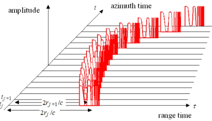
where cis the speed of light. For airborne SARs, the maximum slant-range distance is several tens of km, which is shorter than the slant-range of spaceborne SARs and a return signal is received before the next pulse transmission. However, for spaceborne SARs, slant-range is very long and a return signal is received not before the next pulse transmission but after several pulse transmissions as shown in Figure 2.2.

The other important signal parameter is wavelengthλ, which is related to the radar frequencyf₀ (in Hz) by

λf₀ =c (2.2)

2.2 Image Formation in Range Direction

Most imaging radars, including real aperture radars (RAR) and SAR, achieve high resolution in range direction by using the pulse compression technique. Before the

pulse compression technique was invented, conventional rectangular pulses without frequency modulation were used to produce radar images. In this section, the image formation processes with rectangular pulses and with the pulse compression technique are described.

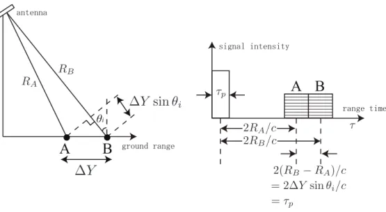
2.2.1 Image Formation with Rectangular Pulses

Consider a side-looking radar transmitting a rectangular pulse of duration τ_p toward a point scatterer “A” and “B” separated by a distance ∆Y on ground-range direction as shown in Figure 2.3. The received pulses from those point scatterers, in principle, take the same rectangular form but with reduced amplitude. The delay between transmission and reception is the time taken for the pulse to travel the two-way distance between the antenna and the scatterer, and it is given by 2R_A/c for the scatterer “A” and 2R_B/c for the scatterer “B”, whereR_Aand R_B are the slant-range distances from the antenna to the scatterer “A” and “B” respectively, and “c” is the speed of light. If the two point images are separated by the time longer than the pulse width, they can be distinguished. If they overlap, then the two point scatterers cannot be resolved. The time resolution is defined as the time duration when the two point images are just separated. This time resolution is the pulse durationτ_p, and the ground-range spatial resolution can be deduced from the relation 2∆Y sinθ_i/c =τ_p, whereθ_i is the incidence angle as illustrated in Figure 2.3. Thus, the spatial resolution in ground-range direction is defined as

∆Y = cτ_p

2 sinθ_i (2.3)

For example, a RAR with pulse duration τ_p = 0.1µs operating at an incidence angle θ_i = 30^◦ has the resolution ∆Y = 30 m, and ∆Y = 3 m withτ_p = 0.01µs. For radars

with rectangular pulses, the shorter the pulse duration is, the finer the resolution becomes. The resolution also becomes coarse as the incidence angle decreases, and

∆Y → ∞ in the limit of θ_i → 0. This is the reason why the imaging radar is side-looking.

A B

θi

JURXQGUDQJH DQWHQQD

A B

VLJQDOLQWHQVLW\

UDQJHWLPH

Figure 2.3: Illustrating range imaging process and resolution of a conventional radar with rectangular pulses.

2.2.2 Image Formation with the Pulse Compression Tech- nique

In the conventional technique based on rectangular (non-chirp) pulses, resolution improves as pulse duration becomes shorter. However, there is a limit to continu- ously generate high-power short pulses using onboard power supply for airborne and spaceborne SARs. To overcome this problem, the pulse compression technique was developed. In this technique, high resolution in range direction can be achieved by using frequency modulated (FM) or chirp pulses of long duration, and by applying appropriate signal processing to received pulses. In particular, for spaceborne SARs

whose power supply is from solar panels, the pulse compression technique is essential and a must. Most of recent airborne SARs also use the pulse compression technique to achieve high resolution in range direction. A unique characteristic of the pulse compression technique is that higher resolution can be achieved with longer pulse duration, contrary to the conventional non-chirp radars.

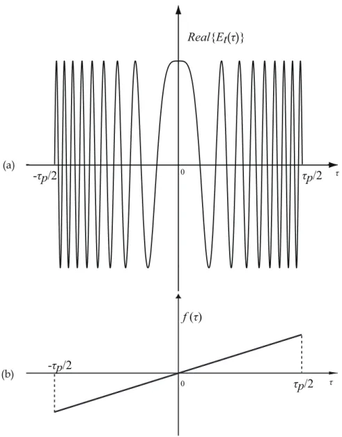
FM pulse or chirp pulse is a pulse whose frequency changes linearly with time τ. The FM pulse (transmitted signal) is defined as follows [1, 2, 30].

E_t(τ) =E₀^′ exp(iω_cτ+iατ²) : |τ| ≤τ_p/2 (2.4)

where E₀^′ denotes the amplitude of the transmitted signal, ω_c denotes the center radian frequency, α is the chirp constant, α/π is called chirp rate or FM rate, and τ_p is the pulse duration. Without a loss of generality, a complex expression is used in Equation (2.4). In practice, the transmitted and received pulses are in a real form, but after pulse reception the real signal is transformed into a complex signal by filtering. It should be noted that in many fields of science and engineering, complex expressions are adopted and the real component is taken from the final expression because of the mathematical complexity of using trigonometric functions. The phase of a charp pulse is ψ(τ) = ωcτ+ατ², and therefore the instantaneous frequencyf can be derived as

f(τ) = 1 2π

dψ dτ

= f_c+ ατ

π (2.5)

and the charp bandwidthB_R can be given as

B_R=|α|τ_p/π (2.6)

f (τ)

Real{Et(τ)}

-τp/2 ⁰ τp/2 ^τ

(a)

(b) τp/2 ^τ

-τp/2

0

Figure 2.4: Illustrating (a) the real component of the phase of a FM pulse and (b) instantaneous frequency withω_c = 0.

The frequency of the chirp pulse varies linearly with time with the gradient α/π.

The gradient is the chirp rate. Figure 2.4 illustrates the charp pulse when the center frequency is 0 Hz. For JERS-1 SAR, α/π = −4.3×10¹¹ Hz/s, τ_p = 35.2 µs, B_R = 15 MHz, f_c = 1275 MHz, and λ= c/f_c = 0.235 m. The positive chirp rate is called up-chirp and the negative chirp rate is called down-chirp. Note that the word “chirp”

stems from “birds’ chirp” in which birds chirp with increasing frequency.

The received signal from a point scatterer at a distance R₀ from the antenna takes

the same form as the transmitted signal but with reduced amplitude and reception time is delayed by 2R₀/c from the time of pulse transmission. The received signal, therefore, is given by

E_s(τ) =E₀exp(i2πf_c(τ−2R₀/c)+iα(τ−2R₀/c)²) : |τ−2R₀/c| ≤τ_p/2 (2.7)

where E₀ is the amplitude of the received signal. Such signal data are called “raw data” because the data do not indicate any imagery yet. After low-pass filtering, the received signal is described as

Es(τ) =E0exp(−i2kR0+iα(τ−2R0/c)²) (2.8)

where k= 2π/λ(λ=c/f_c) is the wavenumber.

Then, in time domain processing, the received signal is correlated with a reference signal which is a complex conjugate of the transmitted signal as expressed below

E_r(τ) = rect(τ /τ_p) exp(−iατ²) (2.9)

where the rectangle function is defined as follows.

rect(τ /τ_p) = 1 : when −τ_p

2 ≤τ ≤ τ_p 2

0 : otherwise (2.10)

The correlation processing is defined as

E_R(τ^′) =

∫ _∞

−∞

E_s(τ^′+τ)E_r(τ)dτ (2.11)

where τ^′ is the time variable in the image plane. Because the phase of the reference

signal is “matched” to the phase of the complex conjugate of the charp (transmitted) signal, the correlation processing of equation (2.11) is called “matched filtering” in time domain. In actual SAR processors, the matched filtering is carried out in the frequency domain so as to produce images from raw data in range direction, i.e., the received signal is Fourier transformed, multiplied by the reference spectrum which is the Fourier transform of the reference signal, and finally the resultant image spectrum is inverse Fourier transformed to produce the image in time (or equivalent space) domain. Here, the matched filtering is introduced in time domain because it is much easier to explain the correlation operation in the time domain. The details of the matched filtering in the frequency domain can be found in [1].

The integral of Equation (2.11) can be solved as

ER(τ^′) =E0exp(−i2kR0)(τp−|τ^′−2R0/c|) sinc[(α(τ^′−2R0/c)(τp−|τ^′−2R0/c|))]

(2.12) where the sinc function is defined as sinc(z) = sin(z)/z. The image plane (origin) of equation (2.12) is at the antenna (the time of pulse transmission). It is convenient to change the origin of the time variable to the image plane at slant-range 2R₀/c as follows (also shown in Figure 2.5).

τ_R=τ^′−2R₀/c (2.13)

Equation (2.12) can then be written in a simpler form

ER(τR) =E0exp(−i2kR0)(τp−|τR|)sinc (ατR(τp−|τR|)) (2.14)

E_R is a complex image amplitude of a point scatterer and is called point spread

Figure 2.5: Change of coordinate origin in slant-range time. (a) Origin at the antenna.

(b) Origin at the ground.

function (PSF) or impulse response function (IRF). The intensity PSF is given by

|E_R(τ_R)|²=|E₀|²(τ_p−|τ_R|)²sinc²(ατ_R(τ_p−|τ_R|)) (2.15)

Here, exp(−i2kR₀) in Equation (2.15) is averaged out as zero since it consists of sine and cosine. Figure 2.6 shows the intensity PSF. The generally accepted definition for SAR resolution is the -3 dB criterion for two-point resolution. The two-point resolution defines the ability of distinguishing the images of two neighbouring point scatterers. According to the -3 dB criterion, the size of the resolution cell (time) ∆τ_R is defined as the distance (time) between two PSFs when the peak of the sum of the two PSFs equals the peak value of a single PSF. In equation (2.15), this distance corresponds to that from the center of the PSF to the position where the PSF has the -3 dB value if the peak value is set to 0 dB. The resolution cell defined by the Rayleigh criterion is the distance from the position of the peak of a PSF to the position of the first zero. In practice, the -3 dB resolution is often approximated by the Rayleigh resolution. The resolution time ∆τ_R based on the Rayleigh criterion can be deduced by solving

α∆τ_R(τ_p−|∆τ_R|) =π (2.16)

-5π

|

|

0 1

ΔY

・・・・・・

・・・・・・

5π π 2π 3π 4π -π

-4π -3π -2π πY

Figure 2.6: Intensity point spread function in range direction.

As a result, the resolution time ∆τ_R is

∆τ_R= τ₀ 2

( 1−

√

1− 4 τ₀B_R

)

(2.17)

where the product of the pulse duration and bandwidth

TBP =τ₀B_R (2.18)

is called TBP (time bandwidth product). The TBP of general SAR systems is large.

For JERS-1 SAR, τ₀B_R = 35.2(µs)×15(MHz) = 528. For large TBP (τ_pB_R ≫ 1), the pulse compression ratio (ratio of pulse duration τ_p to the resolution time ∆τ_R)