RES Discussion Paper Series
No. 5
A Compositional Data Analysis of Market Share Dynamics
Yoshiyuki Arata
Research Institute of Economy, Trade and Industry
Tamotsu Onozaki
Faculty of Economics, Rissho University
December 2018
Rissho Economics Society (RES) Rissho University
4-2-16 Osaki, Shinagawa-ku Tokyo, 141-8602 Japan
A Compositional Data Analysis of Market Share Dynamics ∗
Yoshiyuki Arata
1†Tamotsu Onozaki
21Research Institute of Economy, Trade and Industry
2Department of Economics, Rissho University
Abstract: The existing literature has shown that there are several statistical regularities in indus- trial dynamics, which are an important clue to understanding for the underlying mechanism. This paper focuses on market share changes and shows that its distribution has some remarkable properties. Be- cause of the constrained nature of market share, that is, the sum must be unity, this paper applies the recently developed method calledcompositional data analysis(CDA) to market share data. We find the distribution does not follow a Gaussian but a tent-shaped distribution with a fatter tail, which is closely related with the findings of firm growth rate distribution. With some exceptions, this statistical feature can be observed across different sectors. Furthermore, this property can be observed when we focus on the relation between the top subgroup and lower-ranked firms. This shape of the distribution implies that market share growth cannot be described by an accumulation of small shocks: Rather, lumpy jumps that transform the market structure are crucial in market share dynamics. Put differently, radical change in market structure is a relatively frequent phenomenon. Such implications based on statistical properties of observed data help us further investigate industrial dynamics theoretically.
Keywords: Market share dynamics; Subbotin family; Compositional data analysis JEL Classification Numbers: L22; L11; D43
∗This research was conducted as a part of the Project ‘Sustainable Growth and Macroeconomic Policy’ undertaken at Research Institute of Economy, Trade and Industry (RIETI) and the present paper is based on our prior discussion paper (RIETI Discussion Paper Series 17-E-076, May 2017). This work was partly supported by JSPS KAKENHI (Onozaki:
Grant Number 23330086) and Research Grant of Institute of Economic Studies/Rissho University (Onozaki: 2017).
†Corresponding author, E-mail: [email protected]
1 Introduction
During the past few decades, a series of studies have revealed a number of remarkable statistical regularities in industrial dynamics: the positive skewness and fat-tailedness of firm size distributions (e.g., Axtell (2001), Gabaix (2009)), Laplace shape of firm growth rate distributions (e.g., Stanley et al.
(1996), Bottazzi et al. (2002, 2007, 2011), Bottazzi and Secchi (2006)) and productivity dispersion (e.g., Dosi et al. (2016); for review, see, e.g., Dosi et al. (2017)). Surprisingly, it has been shown that these stylized factsare quite robust and hold across sectors and countries as well as time periods, highlighting universal properties of industrial dynamics. The importance of these statistical regularities cannot be overstated because they give us an important clue to understanding of underlying mechanism. The aim of this paper is to make a contribution to this literature by presenting another new empirical regularity in market share dynamics. Applying a newly introduced statistical method called compositional data analysis(CDA) to Japanese manufacturing firms, we find remarkable distributional features in market share dynamics which have not been addressed in the existing literature.
There has been a strand of literature empirically analyzing market share dynamics (e.g., Geroski and Toker (1996), Davies and Geroski (1997), Mazzucato (2000, 2002), Mazzucato and Parris (2015), and Sutton (2007) ), which gives us insight into how market structure evolves over time.1 This type of analysis, however, is prone to suffer from difficulties caused by the constraint: the sum adds up to unity,
∑D
i=1xi = 1, where xi denotes market share of firmi. In the previous studies, this constraint has not been explicitly taken into account and the conventional multivariate statistical methods developed for theD-dimensional real space RD has been applied to data. However, as explained in the following, this procedure leads to biased results. A constellation of market shares ofDfirms should be viewed as a point on the (D−1)-dimensional hyper-plane given by ∑D
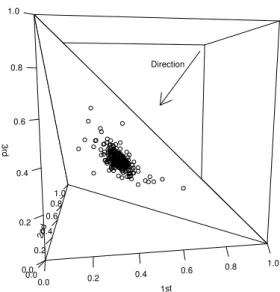
i=1xi = 1 rather than RD. In order for graphical understanding of this constrained nature, a 3-dimensional case (i.e., D = 3) is depicted in Figure 1, where sample points are plotted not inRD but on the triangle representing the planex1+x2+x3= 1.
For an illustration of how this constraint causes difficulties, let us consider correlation analysis as in Sutton (2007), where he examines the correlation coefficient between market share changes of the top 2 firms, finding that it is close to 0. Suppose that there are three firms in a market, each of which has an equal market share, and our focus is to examine the relation between firms 1 and 2. Let Xi and xi, i= 1,2,3 be the sales and the shares of the three firms, respectively (i.e., x1 =x2=x3= 1/3). We assume that the sales of each firm grow independently and the growth rate follows a normal distribution:
The sales of a firm in the next year are given by εiXi andεi is drawn fromN(1, σi2). Since the growth rates,ε1 andε2, are drawn independently, the sample correlation coefficient is close to 0 (see Figure 2, in which Corr(ε1, ε2) =−.000790). Thus, the sample correlation coefficient gives us an insight into the
1Among them, Sutton (2007) is closest to the aim of this paper. Sutton (2007) uses a large and disaggregated data set on Japanese manufacturing firms and tries to find new statistical regularities that holds universally.
1st
0.0 0.2 0.4 0.6 0.8 1.0
2nd
0.0 0.2
0.4 0.6
0.8 1.0 3rd
0.0 0.2 0.4 0.6 0.8 1.0
Direction
Figure 1: 3-dimensional case.
underlying mechanism.
0.7 0.8 0.9 1.0 1.1 1.2 1.3
0.70.80.91.01.11.21.3
Firm 1
Firm 2
Figure 2: Scatter plot of sales growth, ε1 and ε2. In this simulation, σ1 =σ2 =.1 and the number of samples is 500. The sample correlation coefficient is−.000790.
How about market share? Given the sales of the three firms and their growth rates, the growth rate of market shares, ε∗i, can be obtained as follows: for each i,ε∗i := ∑ εiXi
j=1,2,3εjXj/xi= ∑ 3εi
j=1,2,3εj because of the equal market shares. The sample plots of ε∗1 and ε∗2 with different values of σ3 and correlation coefficients are given in Figure 3. Panel (a) and (b) in Figure 3 suggests that whenσ3is not large, that is, the variance ofε3 is not large, the sample correlation coefficient shows a negative value even though the growth rates ofsalesare independent with each other as shown Figure 2. This is due to a negative bias by the constraint of market share because an increase in a firm’s share must be offset by decreases
in other firms’ shares.2
In contrast, whenσ3is large, the market shares of firms 1 and 2 have to increase and decrease together to offset the fluctuation of the firm 3 market share. Because of this effect, the sample correlation coefficient becomes positive, Corr(ε∗1, ε∗2) =.580, as shown in Figure 3(c). Note that the underlying relation between firms 1 and 2 is exactly the same as in Figure 2, that is, independence. Since these positive and negative values of sample correlation coefficients are caused by the constraint, it is seriously misleading to interpret them as an evidence of some economic mechanism. The point is that the bias depends on the behavior of firm 3 even if our focus is on the relation between firms 1 and 2. Since the correlation coefficient is biased to the unknown extent, it is impossible to obtain implications about firms’ relation from the correlation analysis.3 Given the fundamental role of correlation coefficient in statistical analysis, this suggests that we need an alternative approach to uncover empirical regularities in market share dynamics.
0.25 0.30 0.35 0.40
0.260.280.300.320.340.360.380.40
Firm 1
Firm 2
(a) σ3=.01.
0.25 0.30 0.35 0.40
0.300.350.40
Firm 1
Firm 2
(b)σ3=.1.
0.20 0.25 0.30 0.35 0.40 0.45 0.50 0.55
0.200.250.300.350.400.450.50
Firm 1
Firm 2
(c)σ3=.4.
Figure 3: Scatter plot of market share growth, ε∗1 andε∗2. The sample correlation coefficients are given by (a)−.798 (b)−.526 and (c).580, respectively. Note that the sales of the two firmsε1 andε2 used to obtainε∗1andε∗2are exactly the same as the ones in Figure 2. The only difference inσ3yields differences in these panels.
To overcome these difficulties, we introduce CDA in this paper, which enables us to obtain implications of market share dynamics without the bias mentioned above. In particular, by defining new operators, CDA enables us to use statistical concepts such as mean, variance, distribution and the central limit
2Formally, this bias is described as follows. From the constraint and its expectation, we have x1−E[x1] +x2−E[x2] +...+xD−E[xD] = 0.
By multiplying both sides of this equation byx1−E[x1] and taking expectation, we obtain Var(x1) + Cov(x1, x2) +...+ Cov(x1, xD) = 0
Cov(x1, x2) +...+ Cov(x1, xD) =−Var(x1) (<0), where Var and Cov denote the variance and covariance, respectively.
3One might say that this difficulty can be avoided by using data free from such a constraint as∑n
i=1xi= 1. Indeed, Coad and Teruel (2012) follow this strategy and inspect firm growth measured by employees, sales, and value added instead of market share. They find the uncorrelated growth rates of rival firms, consistent with Sutton’s finding. However, another problem arises concerning this type of analysis. Let us suppose a market whose size fluctuates due to demand shocks.
Market expansion and contraction may lead to the comovement of sales of firms and a positive correlation between sales, but this positive correlation cannot be interpreted as evidence of a complementary relation between rival firms. In other words, even a fiercely competitive relationship can be positively biased due to the fluctuation of market size.
The point in our analysis is that we focus on therelativemarket position: Market share captures how a firm’s position changescompared with its rivals.
theorem on the space of market shares. We apply CDA to market share data on Japanese manufacturing firms and explore statistical properties of market share dynamics. To the best of our knowledge, this paper is the first application of CDA to the comprehensive market share data.
Our analysis shows that the distribution of market share change displays a remarkable feature: The distribution does not follow a Gaussian but a Laplace-like tent-shaped distribution with a fatter tail.
This distribution is closely related with the findings of firm growth rate distribution. This shape of the distribution implies that market share change cannot be described by an accumulation of small shocks. Rather, lumpy jumps than completely transform the market structure are crucial in market share dynamics. Namely, such a radical change in market structure is relatively frequent. Interestingly, with some exceptions, this statistical feature can be observed across different sectors. Furthermore, this property can be observed when we focus on the relation between the top subgroup and lower-ranked firms. Therefore, our analysis shows that this statistical property captures an essential feature of market share dynamics.
The rest of paper is organized as follows. Section 2 introduces CDA and shows its applicability to the analysis of market share dynamics. Section 3 applies CDA to market share data of Japanese manufacturing firms. In particular, Section 3.2 analyzes the top 2 firms and explore its distributional properties. Section 3.3 extend our analysis to the multivariate case (the top 5, 6, and 7 firms) and analyze its marginal distribution. Section 4 concludes this paper. Appendix A summarizes the method of outlier detection employed in our analysis.
2 Compositional Data Analysis (CDA)
CDA is a rapid growing field in statistics and explicitly takes into account the fact that the components sum up to unity: x1+x2+...+xD= 1. The difficulty concerning correlation discussed above is called spurious correlation, which is firstly pointed out by Pearson (1897). The spurious correlation is by no means pathological in real applications. In the field of geology, which is one of the main application fields of CDA, a series of papers (e.g., Chayes (1960)) have confirmed that the spurious correlation is widespread in the literature. Given the importance of compositional data and the obvious constraint, it is surprising that problems related to the spurious correlation have remained unnoticed in other fields including economics.4 The spurious correlation becomes serious especially in the analysis of market share. Suppose that our interest lies in whether the properties of the dynamics of market share depend on market concentration, which is one of the fundamental issues in the early literature (see the Introduction).
However, it is problematic to compare the correlation coefficients with different concentrations because the bias by the constrained nature of market share also depends on the concentration. There is no easy
4One exception in the economic literature is a series of studies by Fry et al. (1996, 2000), in which they apply CDA to budget share models of households’ expenditure. However, to our knowledge, no study has applied CDA to market share data in the existing literature on industrial organization.
way to distinguish correlation representing the underlying economic relation from the bias.
Related to the spurious correlation, the identification of the boundary of relevant markets is another problem which makes an analysis based on the conventional correlation questionable. While the boundary of a market has been explicitly given in most of the theoretical studies and its identification has been viewed as a technical one, this problem turns out to be serious to empirical researchers.5 Moreover, it is in practice unavoidable that some firms are missing, which means that the boundary of a market is misspecified. Any reliable analysis of market share should be robust to the misspecification of a boundary, but the conventional correlation does not satisfy this property. In contrast, CDA overcomes these difficulties in a consistent manner.
In the 1980s, a series of papers in the statistical literature have tackled the difficulties of composi- tional data and these efforts have culminated in the seminal work by Aitchison (1986), who develops an axiomatic approach satisfying a set of fundamental principles. Among them, a principle calledsubcom- position coherencein CDA literature is worth mentioning in our analysis. A subcomposition is defined to be a subset of components; for example, if there areD firms in a market and we haveD shares of firms, x1, x2, ..., xD, ∑D
i=1xi = 1, the shares of two firms,x′1:=cx1, x′2:=cx2, x′1+x′2= 1, where a constant cis introduced so that the sum is unity, is a subcomposition of the full composition. The subcomposition coherence means that results obtained from the subcomposition are coherent with those obtained from the full composition. The conventional correlation does not satisfy this principle whereas CDA does, which is one of our motivations to use CDA. In the 2000s, the approach has been further elaborated and generalized by several statisticians (for reviews, see Pawlowsky-Glahn and Buccianti (2011), Pawlowsky- Glahn et al. (2015)). Following this line of literature, we apply CDA to market share dynamics in this paper.
Let us begin with notations. We define a sample space called simplexas follows:
SD:=
{
x= (x1, x2, ..., xD) :xi>0(i= 1,2, ..., D),
∑D
i=1
xi= 1 }
As noted above, the difficulties related to compositional data arise from the fact that the structure ofSD is different from that of the real sapceRD. For example, the simplex is not a vector space with + and· : ∃x,y∈ SD anda∈Rsuch that ax+y∈ S/ D. It means that we cannot discuss a linear combination such as linear regression and principal component analysis because a linear combination may not be an element in SD. Namely, the operations, + and ·, are not suited for SD. What are operations in SD playing the role of + and· in RD? These operations calledperturbation (denoted by⊕) and powering (⊙) are defined as follows:
5See, e.g., Kaplow (2015). It is common that the boundary of a market is defined in terms of competition, that is, firms are in a market if they compete against each other. However, competition is a concept difficult to define and sometimes depends on the boundary itself.
x⊕y:=C(x1y1, x2y2, ..., xDyD), α⊙x:=C(xα1, xα2, ..., xαD), Cx:=
( x1
∑D
i=1xi, x2
∑D
i=1xi, ..., xD
∑D i=1xi
) ,
where the operationC is calledclosure.
It should be noted that the two operations⊕and⊙have economic meaning, especially in the context of firm growth models. Suppose that the firm growth process follows Gibrat’s law, that is, the sales of firmi,si,t, grow proportionally to its previous sales:6
si,t=εi,tsi,t−1, (1)
where εi,t is a growth shock independent from its previous sale. Exprssing sales of firms in terms of market share (i.e.,xt:=C(st)), equation (1) is written as follows:
xt=xt−1⊕εt.
Thus, the sharesxtcan be seen as thesumof the previous shares and a growth shock with the operation
⊕. As in the same manner, thedifferenceof shares between successive years can be defined as follows:
xt⊖xt−1:=xt⊕(−1)⊙xt−1=εt.7
As in the conventional linear regression and principal component analysis, the orthogonality needs to be defined inSD for further analysis. We introduce Aitchison inner product inSD as follows:
⟨x,y⟩A:= 1 D
∑
i<j
log xi xj
logyi yj
The induced distance is given by
dA(x,y) :=∥x⊖y∥A=
√1 D
∑
i<j
( logxi
xj −log yi yj
)2
The meanings of the inner product and distance become clear by considering a transformation fromSD toRD. First, we define thecentered log-ratio(clr) transformation:
6In the literature on firm growth, it is well-known that Gibrat’s law provides a good fit to empirical data, especially for large firms. See, e.g., Coad (2009).
7In a different strand of literature, a replicator model is used to describe the path of firm growth (see, e.g., Mazzucato (2000), See ICC Dosi et al 2017 footnote 4 ):
dsi,t
dt =λisi,t, st=s0·exp(λt),
where λ= {λ1, λ2, ..., λD} is a constant vector representing the competitiveness of firms. The equation above can be written in terms of⊕and⊙as follows:
xt=x0⊕t⊙exp(λ).
Thus, the replicator model can be seen as astraight lineinSDwith angle exp(λ).
v= clr(x) := log [ x1
gm(x), x2
gm(x), ..., xD gm(x)
]
, gm(x) = (∏D
i=1
xi )
with inverse,
x= clr−1(v) :=Cexp(v).
The clr transformation has several useful properties; for example, it preserves the structure given by perturbation and powering, that is,
clr((α⊙x)⊕y) =αclr(x) + clr(y).
Furthermore, the Aitchison inner product and distance can be simplified by the clr transformation:
⟨x,y⟩A=⟨clr(x),clr(y)⟩, dA(x,y) =d(clr(x),clr(y)) = vu ut∑D
i=1
(clri(x)−clri(y))2,
where ⟨·,·⟩ and d(·,·) are the usual inner product and Euclidean distance in RD, respectively. Thus, by the clr transformation, ⊕, ⊙, ⟨·,·⟩A, and dA(·,·) in SD correspond to +, ·, ⟨·,·⟩, and d(·,·) in RD, providing a Euclidean structure toSD. This means that we are able to deal with elements in SD as if they are variables inRD with the usual operations. However, it should be noted that clr(x) has a new constraint,∑D
i=1clri(x) = 0, that is, the transformed data are collinear. To overcome this disadvantage, Egozcue et al. (2003) introduce theisometric logratio (ilr) transformation.
The ilr transformation is essentially equivalent to choosing an orthonormal basis on the hyperplane H :={v∈RD:∑D
i=1vi = 0}by, for example, the Gram-Schmidt algorithm. Formally, this is defined as follows: let{e1,e2, ...,eD−1}be an orthonormal basis ofSD, i.e.,⟨ei,ej⟩A=δij. For a fixed orthonomal basis, the ilr transformation is given as follows:
x∗= ilr(x) := (⟨x,e1⟩A,⟨x,e2⟩A, ...,⟨x,eD−1⟩A) x= ilr−1(x∗) :=⊕Di=1−1x∗j⊙ei.
The ilr transformation gives the coordinates ofxrepresented inRD−1. Analogous to the clr transforma- tion, the ilr transformation satisfies the following relations:
ilr((α⊙x)⊕y) =αilr(x) + ilr(y).
⟨x,y⟩α=⟨ilr(x),ilr(y)⟩, dα(x,y) =d(ilr(x),ilr(y))
Note that x ∈ SD is transformed into x∗ ∈ RD−1 by ilr and x∗ has no additional restriction. x∗ is a
variable inRD−1 and therefore the conventional multivariate statistics inRD−1 can be directly applied tox∗. In short, our strategy consists of the following steps (see Table 1):8
1. Variables in SD, that is, market share in our analysis, are transformed intoRD−1by ilr.
2. Multivariate statistical analysis in RD−1 (e.g., principal component analysis (PCA) and cluster analysis) are carried out on the transformed variables.
3. The results are inversely transformed to the original space SD by ilr−1.
ilr ilr−1
SD =⇒ RD−1 =⇒ SD
Compositional data Multivariate statistical analysis Interpretation Table 1: Working on coordinates.
In the next section, market share dynamics is examined based on this strategy.
3 Market Share Dynamics
3.1 Data
Our dataset consists of annual observations of market shares of Japanese manufacturing firms over the period of 1980–2009. The source of our data isMarket Share in Japan, published by Yano Research Institute Ltd.9 The classification corresponds roughly to 6-digit commodity classification for the Census of Manufactures in Japan, in which manufacturing goods are classified into 2,363 markets.10 This source is unique in that the unit of analysis is market: we obtain market composition and the names of firms for each market. While databases used in previous works (e.g., Coad and Teruel (2012)) have detailed information on firms’ attributes, firms are classified to a single sector according to their main activity.
However, not a few firms, especially large firms, supply more than one product. In contrast, our database focus on markets rather than individual firms, and firms supplying more than one product appear across multiple markets in our dataset.
The choice of markets examined in our analysis is based on two criteria: the length of the time series and the number of firms in a market. Since we focus on markets existing over a long period rather than emerging or disappearing markets, we restrict our attention to markets with more than 25-annual observations over the period of 1980–2009.The sectors and the number of markets examined in our analysis are given in the following sections.
8This strategy is called the principle of working on coordinates in the CDA literature. See, e.g., Mateu-Figueras et al.
(2011).
9This data source is the same one used in Sutton (2007) and Kato and Honjo (2006).
10Hereafter, we call 6-digit classificationmarkets(e.g., heavy bearing rings) and 3-digit classification (e.g., iron & steel) sectors.
3.2 Distribution of market share growth
In this section, we focus on the top 2 firms and examine market share growth defined byεt:=xt⊖xt−1. As we have discussed above, we can define the distribution of market share growth by CDA. Based on this method, we explore its distributional properties in the following analysis.
We first transformε= (ε1, ε2) in S2 into a one-dimensional variable inRby the ilr transformation:
ilr(ε) = √1 2log(εε1
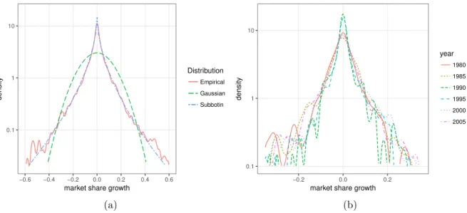
2).11 Figure 4(a) shows the kernel density estimate of pooled market share growth, ilr(ε), over 1980–2009, aggregated across over all the sectors. Descriptive statistics is given in Table 2.
The first to be noticed is that the mean of ilr(ε) is very close to 0, which corresponds to the neutral elementλ2= (12,12) inSD. Sinceε=λ2does not change its relative position in the next year, that is, x⊕λ2 =x, market share growth is on average like a fair coin tossing: The chances of taking market share away from its rival are fifty‐ fifty. Regarding distributional properties, Figure 4(a) clearly suggests the significant departure from normality:12 Rather, the distribution is leptokurtic (tent-shape) and has fatter tail than that of Gaussian distribution. Namely, compared with a Gaussian distribution, we often observe drastic change in market structure with non-negligible probability. Moreover, this shape of the distribution is stable over time: Figure 4(b) plots kernel density estimates of ilr(ε) in different years, showing similar tent-shaped distributions.
This finding is closely related tostylized factsof the distribution of firm growth rates. In the existing literature, it is empirically known that the distribution of firm growth rates does not follow a Gaussian but a Laplace distribution, which is similar to the one shown in Figure 4.13 Interestingly, this statistical feature is observed at a disaggregated level and the shape of distributions across different sectors shows a surprising degree of homogeneity. This remarkable regularity implies that firm growth cannot be described by an accumulation of small independent shocks: if firm growth is a consequence of many small shocks, the distribution of firm growth rate would be Gaussian by the central limit theorem, which contradicts the stylized fact. Rather, the Laplace shape and the fatter tail implies that firm growth is characterized by lumpy jumps: Namely, drastic change in market structure is not rare but relatively common.
While the relationship with rivals is not taken into account in the literature on the distribution of firm growth rates, Figure 4 captures the statistical properties of change in relative market position. The same argument as in firm growth rates applies to the market share growth: market share dynamics cannot be characterized by gradual and smooth change. Rather, significant episodes of complete transformation of the market structure are relatively frequent.
11The explicit form of the ilr representation is obtained as follows. First, we transformεby the clr transformation:
clr(ε) = (loggε1
m(ε),loggε2
m(ε)) with loggε1
m(ε)+ loggε2
m(ε) = 0. Second, we choose an orthonormal basis in this space. Since the dimension of this space is 1, the choice of an orthonormal basis is either √1
2(1,−1) or √1
2(−1,1) inR2. The former is chosen here. Finally, taking an inner product with this basis, we obtain the ilr representation ofε, ilr(ε) = √1
2log(εε1
2).
12The null hypothesis of normality is rejected at 1 percent significance level by Anderson-Darling normality test.
13See a series of papers by G. Bottazzi and his coauthor (e.g., Bottazzi et al. (2002, 2007, 2011)). For theoretical explanations of the Laplace distribution, see Bottazzi and Secchi (2006) and Arata (2014).
0.1 1 10
−0.6 −0.4 −0.2 0.0 0.2 0.4 0.6
market share growth
density
Distribution Empirical Gaussian Subbotin
(a)
0.1 1 10
−0.2 0.0 0.2
market share growth
density
year 1980 1985 1990 1995 2000 2005
(b)
Figure 4: Kernel density estimation and fitted density functions. In (a), market share growth over the period 1980–2009 is pooled. “Empirical” refers to the kernel density estimation with Gaussian kernel.
Bandwidth is chosen following the method in Scott (1992), using factor 1.06. “Gaussian”(“Subbotin”) refers to the Gaussian (Subbotin) fit. In (b), kernel density estimations in 5 different years are plotted.
Estimation method is the same as in (a).
To further characterize the shape of the empirical distributions, we consider a family of distributions calledSubbotindistributions, which are used to describe firm growth rate distribution (see, e.g., Bottazzi and Secchi (2006)). The probability density function of Subbotin distributions is given as follows:
p(x) := 1
2ab1bΓ(1 + 1/b)exp
(−(|x−µ|b) bab
)
, (2)
where µis a location parameter,ais a scale parameter, and b represents the shape of the distribution.
Subbotin family includes Gaussian (b = 2) and Laplace distributions (b = 1) as special cases. Thus, a smaller value of b, especiallyb < 2, indicates the fatness of the tail. Maximum likelihood estimates (MLE) of aand b are reported in Table 2. This shows that the parameterb is not only lower than 2 (Gaussian case) but lower than 1 (Laplace case).14 The tail of ilr(ε) is significantly fatter than that of a Laplace distribution. As noted above, leptokurticity and fat-tailedness are remarkable characteristics of the distribution of market share growth.
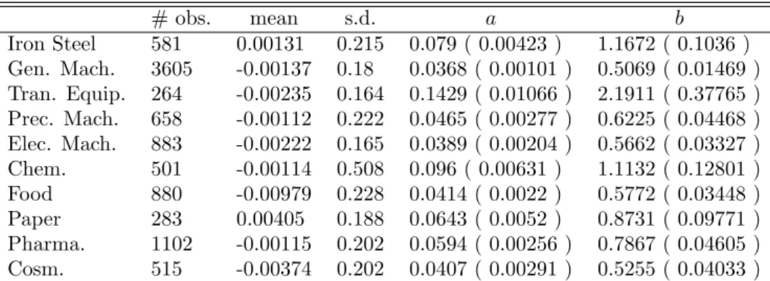
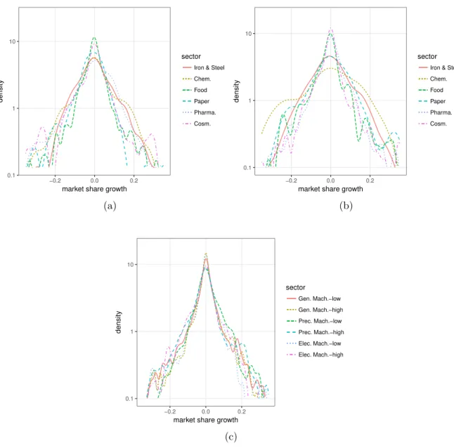
Next, we analyze this shape of the distribution at more disaggregated level, that is, each of the 10 3-digit sectors are considered separately. In Figure 5, all the 30 years of market share growth are pooled together under the stationary assumption. MLEs for each sector are given in Table 3. Figure 5 and Table 3 show that the distribution in all sectors except Transportation Equipment is tent-shaped as in the aggregate case: the parameter b is close to or smaller than 1. While we can observe some heterogeneity across sectors, especially Gaussian shape in Transportation Equipment, we can say that
14The null hypothesis ofb= 1 is rejected for all cases at 1 percent significant level by the loglikelihood ratio test.
# obs. mean s.d. a b Pooled 9273 -0.00189 0.222 0.0448 ( 0.00076 ) 0.5507 ( 0.0112 ) 1980 296 -0.00232 0.109 0.0464 ( 0.00385 ) 0.6986 ( 0.06988 ) 1985 290 -0.01407 0.149 0.0524 ( 0.00433 ) 0.7737 ( 0.08236 ) 1990 308 -1e-05 0.089 0.0253 ( 0.00245 ) 0.4455 ( 0.04333 ) 1995 311 0.01124 0.128 0.0314 ( 0.00283 ) 0.5294 ( 0.05017 ) 2000 320 0.00631 0.093 0.0498 ( 0.00399 ) 0.6957 ( 0.0683 ) 2005 325 0.00563 0.114 0.0493 ( 0.00401 ) 0.673 ( 0.06651 )
Table 2: Descriptive statistics and MLE. The 5th and 6th column shows the MLEs of the parametera andb(standard error in parenthesis).
a tent-shaped distribution can be observed at a disaggregated level and the tent-shape observed at the aggregated level is not a mere statistical effect of aggregation. In most of the sectors, drastic and radical change in market structure is a frequent phenomenon.
0.1 1 10
−0.2 0.0 0.2
market share growth
density
sector Iron & Steel Gen. Mach.
Tran. Equip.
Prec. Mach.
Elec. Mach.
0.1 1 10
−0.2 0.0 0.2
market share growth
density
sector Chem.
Food Paper Pharma.
Cosm.
Figure 5: Kernel density estimations. Market share growth over the period 1980–2009 are pooled under the assumption that the distributions are stationary.
Finally, we use the variance ofεas an index of market mobility and examine its relation with market concentration.15 In a strand of literature focusing on evolutionary aspects of market structure (e.g., a series of studies by Mazzucato), the variability of market share (i.e., market mobility) and market concentration are viewed as important indexes characterizing the evolutionary stage of a market.16 In
15The variance ofεcan be defined based on the Aitchison distance:
Var[ε] := 1 D
∑
i<j
Var [
logεi
εj
]
=
∑D
i=1
Var[clri(ε)]
=
D−1∑
i=1
Var[ilri(ε)]
Thus, this is the variance of the transformed data ilr(ε) inRD−1. For later purpose, the variance is defined in a more general form. ForD= 2, the first line of the equation above becomes Var[ε] =12Var
[ logεε1
2
] .
16For example, in an early stage, there are many firms in a market, that is, low market concentration and market share
# obs. mean s.d. a b Iron Steel 581 0.00131 0.215 0.079 ( 0.00423 ) 1.1672 ( 0.1036 ) Gen. Mach. 3605 -0.00137 0.18 0.0368 ( 0.00101 ) 0.5069 ( 0.01469 ) Tran. Equip. 264 -0.00235 0.164 0.1429 ( 0.01066 ) 2.1911 ( 0.37765 ) Prec. Mach. 658 -0.00112 0.222 0.0465 ( 0.00277 ) 0.6225 ( 0.04468 ) Elec. Mach. 883 -0.00222 0.165 0.0389 ( 0.00204 ) 0.5662 ( 0.03327 ) Chem. 501 -0.00114 0.508 0.096 ( 0.00631 ) 1.1132 ( 0.12801 ) Food 880 -0.00979 0.228 0.0414 ( 0.0022 ) 0.5772 ( 0.03448 ) Paper 283 0.00405 0.188 0.0643 ( 0.0052 ) 0.8731 ( 0.09771 ) Pharma. 1102 -0.00115 0.202 0.0594 ( 0.00256 ) 0.7867 ( 0.04605 ) Cosm. 515 -0.00374 0.202 0.0407 ( 0.00291 ) 0.5255 ( 0.04033 )
Table 3: Descriptive statistics and MLE. Thus, this is the variance of the transformed data in RD−1. The 5th and 6th column shows the MLEs of the parameteraandb (standard error in parenthesis).
particular, in order to describe market mobility, several indexes have been used in the literature (e.g., market share instability in Mazzucato (2002)) but suffer from the bias caused by the constrained nature of market share. In contrast, the variance ofεcaptures the variability of market share by definition and is free from the bias by virtue of CDA.
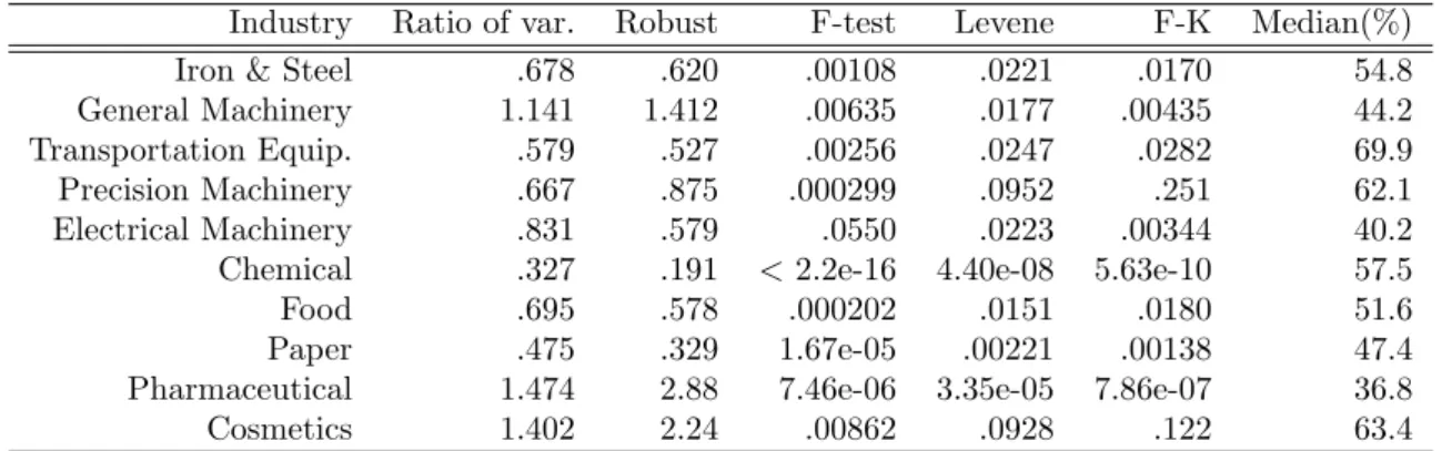
In order to examine the dependence of the variance on its concentration, we decompose our sample data ofεfor each industry by the median of its concentration. Here, the concentration is defined to be the sum of shares of the two firms. Obtaining the two subsets with higher and lower concentrations, we compare the two variances. The results are given in Table 4. Roughly speaking, the results in Table 4 shows that these sectors can be classified into three groups:
• Group 1: Iron & Steel, Transportation Equipment, Chemical, Food, and Paper. The variance of the growthεbecomes larger when market concentration is high.
• Group 2: General Machinery, Precision Machinery, and Electrical Machinery. The variance is less dependent on market concentration.17
• Group 3: Pharmaceutical and Cosmetics. The variance becomes larger when market concentration is low.
While these two market indexes are important to describe the status of market, we cannot find a simple relationship between these two indexes in our analysis. The inter-sectoral heterogeneity of the relation between is quite large: Group 1 shows a positive relationship and Group 3 shows a negative relationship.
In contrast, as shown in Figure 6, in which kernel density estimation of the two subgroups are plotted, we can observe tent-shaped distributions in both subgroups (i.e., high and low concentrations), similar to the ones in Figure 5. In this sense, the tent-shaped distribution is a rather robust feature of market share
is instable (e.g., high entry-exit rate). As it become mature, market competition forces inefficient firms out of the market (high market concentration) and their market shares become stable.
17While the tests for general machinery show the statistically significant difference of the two variances by the large number of observations, the point estimates show that the difference is relatively small. Thus, general machinery is classified into group 2. Precision machinery is classified into group 2 because its robust estimates of the ratio (.875) is relatively close to 1.
dynamics. Specifically, Figure 6(c) shows the kernel density estimates of sectors in Group 2 and suggests that the shape of the distribution is insensitive with respect to market concentration. Focusing on the sectors in Group 2 and extending our analysis to multivariate cases, we further explore the distributional properties of market share growth.
Industry Ratio of var. Robust F-test Levene F-K Median(%)
Iron & Steel .678 .620 .00108 .0221 .0170 54.8
General Machinery 1.141 1.412 .00635 .0177 .00435 44.2
Transportation Equip. .579 .527 .00256 .0247 .0282 69.9
Precision Machinery .667 .875 .000299 .0952 .251 62.1
Electrical Machinery .831 .579 .0550 .0223 .00344 40.2
Chemical .327 .191 <2.2e-16 4.40e-08 5.63e-10 57.5
Food .695 .578 .000202 .0151 .0180 51.6
Paper .475 .329 1.67e-05 .00221 .00138 47.4
Pharmaceutical 1.474 2.88 7.46e-06 3.35e-05 7.86e-07 36.8
Cosmetics 1.402 2.24 .00862 .0928 .122 63.4
Table 4: Ratio of the two variances and tests for equality. The second column shows the ratio of variances (variance for low concentration markets divided by variance for high concentration markets) based on the classical method. The third column shows the ratio of variances based on a robust method. The fourth column is the p-value derived from the F-test of equality of the two variances. The fifth (sixth) column is the p-value derived from Levene’s (Fligner-Killeen) test. The seventh column is the median of market concentration at which our samples are decomposed.
3.3 Who competes against whom?
We have so far analyzed the univariate case (i.e., market share growth of the top 2 firms). In this section, we extend our analysis to a multivariate case, that is, market share dynamics of the top 5, 6, and 7, and then explore distributional properties of εt :=xt⊖xt−1. By increasing the dimension, we can consider more complex relation among firms. For example, consider the following question: Is an increase in a firm’s share offset by a decrease in the share of anotherparticularfirm? If two particular firms compete for market share against each other, market share change would occur within the two firms keeping other firms’ shares unchanged. To explore such relation among firms, we first perform compositional PCA and cluster analysis toεof the top 5 firms. Based on these results, we examine the marginal distribution ofε. Since these methods implicitly assume homogeneity of covariance structure, we focus on sectors in group 2 based on the results in the previous section: general machinery, precision machinery, and electrical machinery.18 Descriptive statistics are given in Table 5. As in the previous section, the mean ofεis very close to the neutral elementλD:= (D1,D1, ...,D1). On average, the relative market position has no information about market share growth in the next year. In other words, in terms of market share, a market leader has no advantages/disadvantages.
Next, we perform compositional PCA, which is done as follows: We first transformεin S5 to ilr(ε)
18Another reason of this choice is the number of observations in each sector.
0.1 1 10
−0.2 0.0 0.2
market share growth
density
sector Iron & Steel Chem.
Food Paper Pharma.
Cosm.
(a)
0.1 1 10
−0.2 0.0 0.2
market share growth
density
sector Iron & Steel Chem.
Food Paper Pharma.
Cosm.
(b)
0.1 1 10
−0.2 0.0 0.2
market share growth
density
sector Gen. Mach.−low Gen. Mach.−high Prec. Mach.−low Prec. Mach.−high Elec. Mach.−low Elec. Mach.−high
(c)
Figure 6: Kernel density estimations. In (a), kernel density estimations of market share growth with low concentration in Group 1 and 3 are plotted. In (b) kernel density estimations of market share growth with high concentration in Group 1 and 3 are plotted. In (c), kernel density estimations of market share growth of both subgroups in Group 2 are plotted. Estimation method is the same as in Figure 4.
# markets # obs. Mean, 1st 2nd 3rd 4th 5th 6th 7th
Top 5 firms
Gen. Mach. 1843 0.201 0.200 0.199 0.200 0.200
Pre. Mach. 102 0.200 0.199 0.201 0.201 0.199
Elec. Mach. 656 0.199 0.199 0.200 0.201 0.201
Top 6 firms
Gen. Mach. 1052 0.167 0.166 0.165 0.167 0.166 0.170
Elec. Mach. 431 0.165 0.166 0.167 0.167 0.168 0.166
Top 7 firms
Gen. Mach. 483 0.143 0.143 0.141 0.143 0.142 0.145 0.144
Elec. Mach. 212 0.141 0.142 0.143 0.143 0.147 0.141 0.143
Table 5: Descriptive statistics. The first column the number of markets. The second column the number of pooled market share growth. The rest of columns refers to the sample mean represented inSD.
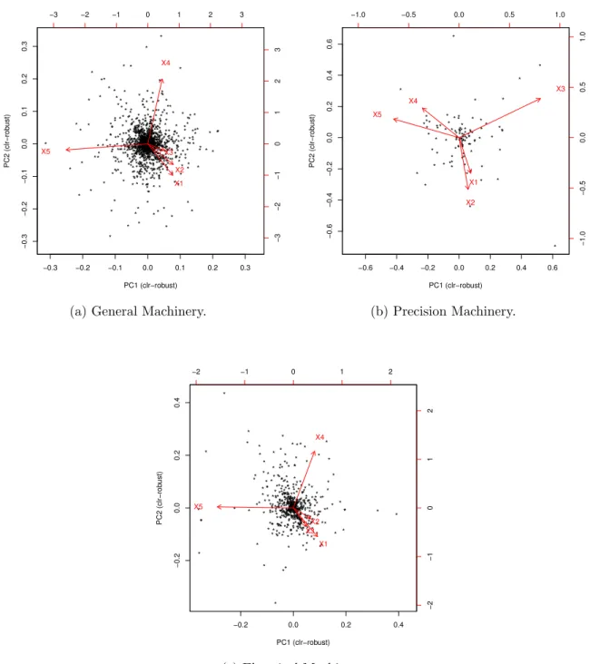
in R4. Next, we apply PCA to ilr(ε), that is, we estimate the location vector and covariance matrix of ilr(ε). Finally, we apply singular value decomposition.19 In this analysis, we focus on two principal components (PCs). Following the convention in the CDA literature, the PCs are inversely transformed to the clr representation for interpretation.
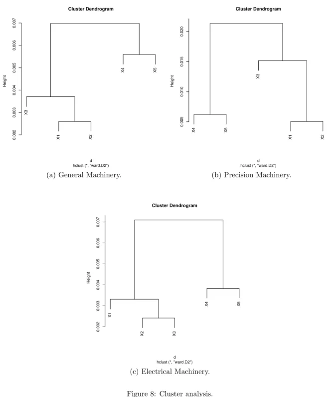
Results are shown in Figure 7. Arrows in these figures represent clr coordinates of the two PCs.20 Figure 7 clearly shows that links betweenε1andε2(andε3) are short, indicating that the shares of firms ranked 1 and 2 (and 3) move up and down together. Namely, when the largest firm succeeds to increase its market share, the market share of the second largest firm is likely to increase and their increases are offset by decrease of the market shares of lower-ranked firms. Put differently, the subgroup of the top 2 (or 3) firms competes against the lower-ranked firms (4th or 5th) for market share. The same picture can be observed by cluster analysis shown in Figure 8.21 Figure 8 shows that the top 2 or 3 firms are clustered as close components and distant from the lower-ranked firms.
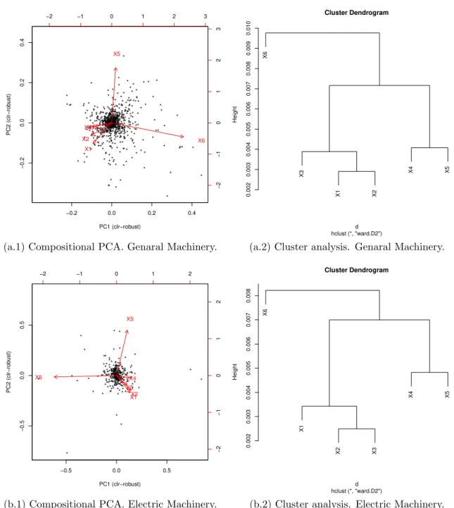
Interestingly, this property can be observed even when we increase the number of firms considered. In Figures 9 and 10, we perform the same analysis with additional firms. Figure 9 shows the compositional PCA and cluster analysis to ε := (ε1, ε2, ...., ε6) of the top 6 firms for general machinery and electric machinery.Figure 10 is the results of the top 7 firms for the same sectors. Both figures show that the shares of the top 3 (or 4) firms are likely to move up and down together. As in the case of 5 firms, the subgroup of the top firms competes against the lower-ranked firms (6th or 7th) for market share.
Next, we examine the distribution of εbased on this finding. While the distribution ofεinSDcan be, in principle, expressed by the corresponding distribution in RD−1, its density estimation becomes practically difficult as the number of dimension increases: Especially when the number of observations is not so large, the density estimation becomes unreliable. Thus, in the remainder of this section, we focus on marginal distributions. As in the usual case in multivariate analysis, there are an infinite number of ways of choosing an orthonormal basis represented in RD. Taking into account the finding above, we consider an orthonormal basis{ei}1≤i≤D−1 whose two elements are given as follows:
e1=
√D−1 D
(
D−1
z }| {
1 D−1, 1
D−1, ..., 1 D−1,−1
)
, e2=
√D−2 D−1 (
D−2
z }| {
1 D−2, 1
D−2, ..., 1
D−2,−1,0 )
Its coordinate represented by this basis is y1 =
√
D−1
D log(ε1ε2...εD−1)
D−11
εD and y2 =
√D−2
D−1log(ε1ε2...εD−2)
D−21
εD−1 . Since these coordinate is the logratio of the geometric mean of the top subgroup to a lower-rankd firm,y1andy2 capture the most variable part ofε. The distributional prop- erties ofy1 andy2 are shown in Figure 11, where we can observe a tent-shaped distribution similar to
19We use a robust method developed by Filzmoser et al. (2009).
20If the clr coordinates of the two PCs are represented as (a1, a2, ..., aD) and (b1, b2, ..., bD), the coordinate of the head of arrowX1 in Figure 7 is (a1, b1).
21Here, the distance between two components is measured by var log(εεi
j), based on which the components are clustered.
For detail, see ...