RES  Discussion  Paper  Series

   

RES  Discussion  Paper  Series  

  No.  1  

       

Chaotic  Itinerancy  in  Regional  Business  Cycle  Synchronization    

Kunihiko  Esashi  

Department  of  Mathematics,  Hokkaido  University    

Tamotsu  Onozaki  

Faculty  of  Economics,  Rissho  University  

Yoshitaka  Saiki  

Graduate  School  of  Commerce  and  Management,  Hitotsubashi  University  

Yuzuru  Sato  

Research  Institute  for  Electronic  Science,  Hokkaido  University  

       

November  2015    

         

Rissho  Economics  Society  (RES)   Rissho  University  

4-­‐‑2-­‐‑16  Osaki,  Shinagawa-­‐‑ku  Tokyo,  141-­‐‑8602  Japan  

Chaotic Itinerancy in Regional Business Cycle Synchronization

Kunihiko Esashi

^∗

Department of Mathematics, Hokkaido University, N10W8, Kita, Sapporo, Hokkaido 060-0810, Japan.

Tamotsu Onozaki

^†

Faculty of Economics, Rissho University, 4-2-16 Osaki, Shinagawa, Tokyo 141-8602, Japan.

Yoshitaka Saiki

Graduate School of Commerce and Management, Hitotsubashi University, 2-1 Naka, Kunitachi, Tokyo 186-8601, Japan.

Yuzuru Sato

Research Institute for Electronic Science, Hokkaido University, N12W6, Kita, Sapporo, Hokkaido 060-0812, Japan.

Abstract

Chaotic itinerancy is complex behavior in high-dimensional dynamical systems characterized by itinerant motion among many different ordered states through chaotic transition. In this study, we robustly observe this behavior in a model of regional business cycles, in which all regions are homogeneous and connected through producers’ adaptive behavior based on global information. Although pro- ducers adjust their output quite slowly toward the average level announced by the government, regional business cycles begin to synchronize due to the entrainment effect. Moreover, the economy is more likely to exhibit chaotic itinerancy when the producers emphasize the expected-profit-maximization and when they adjust their expectations more slowly toward the average. It is also clarified that behind the dynamics of chaotic itinerancy exist cycles among periodic orbits with different unstable directions, which is called unstable dimension variability.

Key words: Regional business cycle, Nonlinear dynamics, Synchronization, Glob- ally coupled map, Chaotic itinerancy, Intermittency, Unstable dimension variability JEL Classifications: C61, E32

∗Present address: NTT DATA Corporation, Toyosu Center Building, 3-3-3 Toyosu, Koto-ku, Tokyo 135-6033, Japan.

†Corresponding author. Phone: +81-3-5487-3021. E-mail address: [email protected].

1 Introduction

Business cycle synchronization has become a topic of growing interest from around the end of the twentieth century (Antonakakis, 2012; Baxter and Kouparitsas, 2005; Yetman, 2011). The vast empirical literature elucidates a fact that countries with intensified trade linkages have resemblant business cycles, which Selover and Jensen (1999) and S¨ ussmuth (2003) explain by proposing a nonlinear mode-locking model. Mode-locking is an inherently nonlinear linkage phenomenon; cycles of different elements are synchronized, i.e., attain mode-lock, when the strength of the linkage between oscillating elements reaches a certain threshold.

On the other hand, with the exception of a stylized fact that fluctuations in different regions of a national economy are inclined to synchronize with each other (Carlino and Sill, 2001; Clark and van Wincoop, 1999; Rissman, 1999), little is known about the busi- ness cycle synchronization across subnational regions within a country, as mentioned by Kouparitsas and Nakajima (2006). One possible hypothesis about subregional synchro- nization is that it may occur due to common exogenous shocks such as national fiscal and monetary policies, sudden changes in world commodity prices, fads among consumers, and so forth. However, several studies find that common shocks do not seem to be the cause of such synchronization (Carlino and DeFina, 1995; Kozlowski, 1995). Another hypothesis is that the synchronization may be caused by trade linkages between different regions of the economy. A nonlinear mode-locking model is again proposed by Selover et al. (2005) under a scenario in which the cycles of different regions synchronize through interregional trade linkages.

It has been well-known that multiple oscillators may synchronize if they directly interact with each other, since the discovery of synchronization of coupled pendulum clocks by Huygens in the seventeenth century. In this sense, a scenario of regional business cycle synchronization through interregional trade linkages is probable and realistic, but rather straightforward and obvious. In contrast, it is also well-known that Southeast Asian fireflies within a given tree (or even larger area) begin to flash simultaneously as night falls. There is no direct interaction among the fireflies; instead, each firefly is considered to sense others’ flashes and adjust its behavior sensitively to the global information. Then an intriguing question arises: do the same mechanisms lie in regional business cycle synchronization? Onozaki et al. (2007) answer this question affirmatively by proposing another hypothesis that regional business cycles may synchronize through producers’ adaptive behavior based on global information which government announces.

They study a system of globally coupled maps (GCM) each of which is nonlinear and may behave chaotically depending on parameter values, and illustrate how synchronization occurs and how complex its process is.    

It would be better to give a short account of a GCM model here, which is first proposed by Kaneko (1990). It is represented as follows:

x

_i

(t + 1) = (1 − ε)f(x

_i

(t)) + ε N

∑

N

j=1

f (x

_j

(t)), i = 1, · · · , N, (1)

where x

_i

(t) denotes the value of the ith element at discrete time period t, and N the num-

ber of elements. A map f(x) describes each element’s endogenous dynamics. Usually a

noninvertible map is utilized as f (x) that may exhibit chaotic behavior. The second term on the right-hand side of (1) represents the global interaction of each element through the mean field, i.e., a uniform, all-to-all interaction. Therefore, two opposite effects coexist:

the all-to-all interaction is inclined to synchronize all elements, and the chaotic instability in each element tends to desynchronize them. Depending on the value of ε ∈ (0, 1), i.e., the balance between these two effects, the GCM model exhibits a rich variety of complex phenomena including chaotic itinerancy (Kaneko, 1990)

¹

. The term describes the phe- nomenon of an orbit successively itinerating among many ordered states through chaotic transitions in dynamical systems. The phenomenon was independently discovered in a model of optical turbulence by Ikeda et al. (1989), a globally coupled chaotic system by Kaneko (1990), and nonequilibrium neural networks by Tsuda (1990). The terminology was coined by its discoverers to denote universal dynamics in a class of high-dimensional dynamical systems (Kaneko and Tsuda, 2000). In an economic context, Yasutomi (2003) studies the emergence and collapse of money in a computer simulation model from the viewpoint of chaotic itinerancy.

In this study, we reexamine the model of Onozaki et al. (2007), and robustly observe chaotic itinerancy for various constellations of parameters as well as various complex phases of regional business cycle synchronization. The remainder of the paper is organized as follows. Section 2 describes a regional business cycle model. Section 3 discusses chaotic itinerancy occurring in the model. Section 4 characterizes chaotic itinerancy compared with of on-off intermittency. The last section concludes the paper.

2 Model

The economy consists of N regions, each with a separate market which is imperfectly competitive. There are many producers in each region, and each producer produces ho- mogeneous goods and delivers them only to the market of its own region. Goods are perishable and cannot be carried over to the next period. Consumers are uniformly distributed over all regions and purchase goods from the market they belong to. We assume that there is no interregional trade in order to concentrate on the effect of pro- ducers’ adaptive behavior based on global information

²

. The government announces the average price and output for all regions in each period, and each producer adjusts its production based on this information; i.e., regions are linked via global information. Each producer decides the next period’s output, considering the average prices and outputs as reference levels. Producer’s decision-making process consists of the following three steps.

First, at period t, each producer in the ith region expects that the actual price p

i

(t) in his market will be adjusted adaptively at period t + 1 toward the announced average

1It is sometimes discussed from the viewpoint of Milnor attractor (Milnor, 1985).

2If considering interregional trade, we have to assume a new economic agent, distributor, who has a behavioral objective completely different from that of producer. This makes the model much complicated and far intractable.

level ¯ p(t) := (1/N ) ∑

_N

j=1

p

_j

(t) with an adjustment speed ε ∈ (0, 1) such that p

^e_i

(t + 1) = p

i

(t) + ε(¯ p(t) − p

i

(t))

= (1 − ε)p

_i

(t) + ε N

∑

N

j=1

p

_j

(t), (2)

where superscript e denotes expectations. Under this price expectation, each producer calculates the output level, ˜ x

_i

(t + 1), maximizing the expected profit subject to the production cost x

²

/2. The resulting amount is

˜

x

_i

(t + 1) = p

^e_i

(t + 1). (3)

Second, each producer dislikes discrepancies between the actual output level at period t, x

_i

(t), and the average level announced by the government, ¯ x(t) = (1/N ) ∑

_N

j=1

x

_j

(t), and intends to resolve them. For this purpose, he sets a provisional target of output ˆ

x

_i

(t + 1) so as to adjust the actual output toward the average level with an adjustment speed ε ∈ (0, 1):

ˆ

x

_i

(t + 1) = (1 − ε)x

_i

(t) + ε¯ x(t)

= (1 − ε)x

_i

(t) + ε N

∑

N

j=1

x

_j

(t). (4)

Third, each producer determines a final output plan as a weighted average of pro- visional target ˆ x

_i

(t) and expected-profit maximizing output ˜ x

_i

(t + 1) with a weight ϕ ∈ (0, 1). The resulting formula is as follows:

x

i

(t + 1) = (1 − ϕ)ˆ x

i

(t + 1) + ϕ x ˜

i

(t + 1)

= (1 − ϕ)(1 − ε) x

_i

(t) + (1 − ϕ) ε x(t) + ¯ ϕ x ˜

_i

(t + 1). (5) Since the sum of the above three coefficients on the right-hand side is unity, we can para- phrase the producer’s decision making as follows: Each producer’s output is determined as a weighted average of x

_i

(t), ¯ x(t), and ˜ x

_i

(t + 1).

The individual demand for each producer’s output is described by a monotonic inverse demand function as follows:

p

_i

(t) = 1

(y

i

(t))

^η

, (6)

where y

_i

(t) is the individual demand and η > 0 is the inverse of the price elasticity of the demand. At each period, prices are determined in each market for equilibrating supply and demand. By substituting (2), (3), (4), and (6) into (5), we obtain a GCM model (1) with a noninvertible map as follows:

f (x) = (1 − ϕ)x + ϕ

x

^η

, (7)

the behavior of which is well studied by Onozaki et al. (2000) and known to exhibit

chaotic behavior depending on a set of parameters. The larger ϕ and η are, the more

likely the economy behaves chaotically. After all, the regional business cycle model to be analyzed in this study consists of (1) and (7).

In what follows, we concentrate on the cases with N = 10 (Section 3) or N = 2 (Sec- tion 4). Unless otherwise noted, η, ϕ, and ε are fixed as 3.5, 0.7, and 0.315, respectively

³

. We randomly select initial conditions x

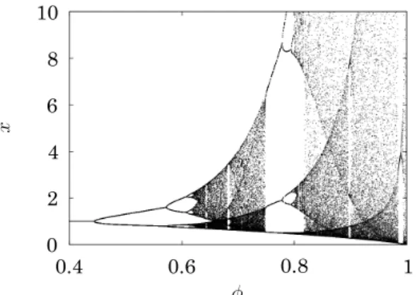
_i

(0) (i = 1, · · · , N ) from the range [0.5, 1.5]. Note that one-dimensional map x(t + 1) = f (x(t)) can generate chaotic behavior through a period-doubling bifurcation as ϕ increases (Fig. 1).

0.4 0.6 0.8 1

0 2 4 6 8 10

x

x

φ

Fig. 1:

Bifurcation diagram of one-dimensional map xt+1 = f(xt) with respect to ϕ. The map can generate chaotic behavior through a period-doubling bifurcation asϕincreases.

3 Chaotic Itinerancy

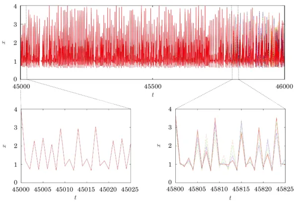
This section investigates chaotic itinerancy in the regional business cycle model (1) and (7). Chaotic itinerancy is a typical phenomenon occurring in high-dimensional chaotic systems. In its presence, an orbit wanders among different states of complexity (Kaneko and Tsuda, 2000). We first show the time developments of the model in Fig. 2. In coupled systems, separate oscillators sometimes synchronize, i.e., a phenomenon called entrainment. A set of synchronizing oscillators is called a cluster. Ten types of regimes (from one-cluster to 10-cluster regime) appear in the model’s behavior. The one- and 10-cluster regimes are shown in Fig. 2 (lower left, lower right).

To characterize chaotic itinerancy, we define the effective dimension and its mean (Komuro, 2005). The effective dimension (ED) of a point x(t) = (x

1

(t), x

2

(t), · · · , x

_N

(t)) ∈ R

^N

with the precision δ, denoted by ED (x(t), δ), is defined simply as a number of clusters. Here, variables within a distance δ are considered to belong to the same cluster

⁴

. We rewrite the model (1) and (7) as a map F : R

^N

→ R

^N

which is defined as follows:

x(t + 1) = F (x(t)).

Then the mean of the effective dimension (MED) of an orbit { x(t) } with the precision δ

3Onozakiet al. (2007) show that the very long transient behavior exists when the system dimension N is fixed as 100 and the parameterη is selected from the range [1.0,8.0].

4The value ofδis fixed as 10⁻⁴ throughout this paper.

Fig. 2:

Time development ofxi(t) (i= 1,· · · ,10) (upper) and its enlargements. The one-cluster regime (lower left) and the 10-cluster regime (lower right) are observed.

for lasting time τ

⁵

is defined as follows:

MED (x, δ, τ ) = 1 τ

τ−1

∑

t=0

ED (x(t), δ).

Because of entrainment effect, synchronization strengthens and the economy remains for some time within the one-cluster regime (ED = 1), which is called a laminar state. Then, the economy leaves the regime and wanders among various regimes, which are called burst states, until coming back to the laminar state. This process is repeated for an extended period (Fig. 3).

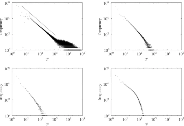
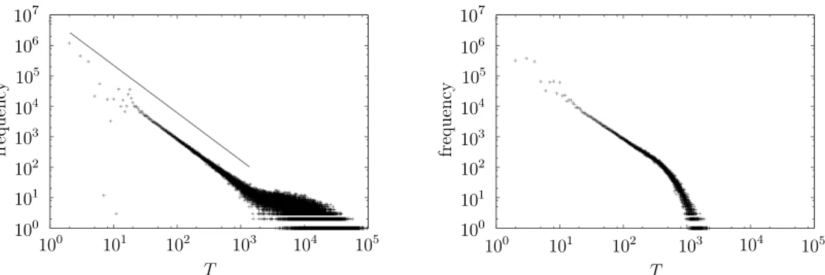
In Fig. 4, the distribution of lasting time within the regime of ED = 1 is shown to obey a power-law with an exponent estimated to be − 3/2 (Heagy et al., 1994)

⁶

. For other regimes of ED = 2, 5, 10 the same distributions are found for shorter periods of time, suggesting that each regime has a mechanism to trap an orbit staying in the regime.

The MEDs of lasting time τ = 10

⁵

are calculated after the transients of 10

⁵

iterations for various εs as shown in Fig. 5. An integer MED indicates that the economy remains in the same regime over 10

⁵

iterations. A non-integer MED indicates that the economy wanders among various regimes of different EDs.

As shown in Fig. 6, we calculate MEDs of the economy by changing a set of parameters (ϕ, ε), and identify the parameter region (ϕ, ε) where MEDs are non-integers, indicating

5The value ofτ is fixed as 10⁵ throughout this paper.

6This kind of power-law distributions are observed in a well-known critical phenomenon called Type III intermittency in a low-dimensional system, but they are not robust in a parameter space. In contrast, the distributions in our model are robustly found.

0 5000 10000 15000 1

2 3 4 5 6 7 8 9 10

ED

Fig. 3:

Time development of effective dimension (ED) of the economy. It primarily remains within the one-cluster regime (ED = 1). Once it departs from the regime, it wanders among various regimes of different EDs until coming back to the one-cluster regime.

10⁶

10⁴

10²

10¹ 10² 10³ 10⁴ 10⁵ 10⁰

10⁰

frequency

T

10⁶ 10⁶

10⁴

10²

10¹ 10² 10³ 10⁴ 10⁵ 10⁰

10⁰

frequency

T 10⁶

10⁶

10⁴

10²

10¹ 10² 10³ 10⁴ 10⁵ 10⁰

10⁰

frequency

T

10⁶ 10⁶

10⁴

10²

10¹ 10² 10³ 10⁴ 10⁵ 10⁰

10⁰

frequency

T 10⁶

Fig. 4:

Distribution of lasting timeT for remaining in a regime of ED (= 1 (upper left), 2 (upper right), 5 (lower left), and 10 (lower right)). The distribution forED= 1 is shown to obey a power-law with an exponent estimated to be−3/2 as indicated by the straight line. For other regimes ofED= 2,5,10 the same distributions are found for shorter periods of time.

that the economy wanders among various regimes

⁷

. Fig. 6 shows the robustness of chaotic itinerancy with respect to large ϕ and small ε. When the producers emphasize

7The MEDs are calculated from 10 randomly chosen initial conditions xi(0) (i = 1,· · · ,10) after neglecting transitions of 10³iterations. If the average is non-integer, the corresponding set of parameters (ϕ, ε) is plotted in Fig. 6. These calculations are performed for 10⁵points in a parameter region (ϕ, ε).

ε

MED

0 0.1 0.2 0.3 0.4 0.5

1 2 3 4 5 6 9 7 8 10

0 0.02 0.04 0.1

ε

0.06 0.08

10−MED

0.01 0.1 1 10

Fig. 5:

The MEDs of lasting time τ = 10⁵ of the economy with respect to ε. A non-integer MED indicates that the economy wanders among various regimes of different clusters (EDs) (left). The graph of 10−MEDforε∈[0,0.1] (right: logarithmic scale) shows that its value is not zero, implying that the orbit wanders among various regimes.

the profit maximization more (larger ϕ) and when they adjust their expectations more slowly toward the average announced by the government (smaller ε), the more likely the economy will exhibit chaotic itinerancy. By comparing the bifurcation diagram of a single map (Fig. 1) with Fig. 6, it is apparent that the model shows complex behavior with multiple regimes around bifurcation points and chaotic regions of a single map. If a single map (7) is nonhyperbolic in some parameter regions, the GCM (1) can easily destroy the respective dynamics of ED = 10

⁸

. This can generate chaotic itinerancy by the extremely small perturbation described by the coupling parameter ε.

φ

ε

1 1

φ

ε

10⁻¹⁰ 10⁻⁷ 10⁻⁴ 10⁻¹

1

Fig. 6:

Parameter region (ϕ, ε) where the economy wanders among various regimes during τ = 10⁵ iterations from 10 initial conditions after the transients of 10⁵ iterations (left). An enlargement of the left figure in logarithmic scale (right).

8Asεis not infinitely small, the same phenomena can be obtained forf(x) having weak hyperbolicity.

4 Detailed Structures of Chaotic Itinerancy

This section focuses on the two dimensional map

⁹

x

₁

(t + 1) = (1 − ε)f(x

₁

(t)) + ε

2 { f (x

₁

(t)) + f (x

₂

(t)) } , x

₂

(t + 1) = (1 − ε)f(x

₂

(t)) + ε

2 { f (x

₁

(t)) + f (x

₂

(t)) } ,

where f(x) is the same map as (7), and studies chaotic itinerancy especially from the view- point of routes between synchronized and desynchronized states in subsection 4.2 (Alexan- der et al., 1992) and the unstable dimension variability in subsection 4.3 (Kostelich et al., 1997; Bonatti et al., 2005). This is because complex behavior wandering among multiple states is observable even in a two dimensional map, which is called the on-off intermit- tency (Fujisaka and Yamada, 1983a, b; Pikovsky and Grassberger, 1991; Glendinning, 2001). We first discuss this point in the next subsection.

4.1 Behaviors in the Two Dimensional Map

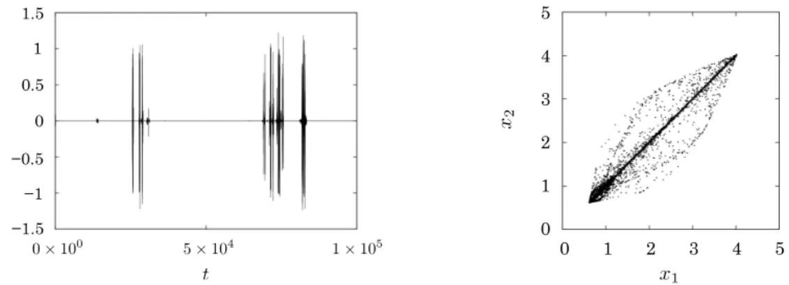
Time series of x

₁

− x

₂

are depicted in Fig. 7 (left), showing the on-off intermittency between a synchronized state (ED = 1) and a desynchronized state (ED = 2). The former is a laminar state where a point (x

₁

, x

₂

) stays in the diagonal line (x

₁

= x

₂

), and the latter a burst state where a point (x

₁

, x

₂

) deviates from the diagonal line (x

₁

̸ = x

₂

) (Fig. 7 (right)).

−1.5

−1

−0.5 0 0.5 1 1.5

1 2 3 4 5

0 0 1 2 3 4 5

Fig. 7:

Time series ofx1−x2(left). Phase space dynamics in (x1, x2) plane (right). On-off intermittency between a synchronized (laminar) state and a desynchronizwd (burst) state is observed.

Next we shed light on the lasting time of laminar and burst states as seen in the ten dimensional map. The distribution of laminar lasting time in a regime of ED = 1 is shown to obey a power-law with an exponent estimated to be − 3/2 (Fig. 8). For ED = 2 the same distribution can be found for the shorter period of time. The results are qualitatively the same as the cases for the ten dimensional map (Fig. 4). Fig. 9 shows a parameter region where the system shows chaotic itinerancy. This also implies that

9This is identical to the ten dimensional map (N = 10) where the initial conditions are given as x1(0) =x3(0) =x5(0) =x7(0) =x9(0) and x2(0) =x4(0) =x6(0) =x8(0) =x10(0). If (x1(t), x2(t)) is the solution, (x2(t), x1(t)) is also the solution due to the symmetry inside the system.

10⁴

10²

10¹ 10² 10³ 10⁴ 10⁵ 10⁰

10⁰

frequency

T 10⁶

10¹ 10³ 10⁵

10⁴

10²

10¹ 10² 10³ 10⁴ 10⁵ 10⁰

10⁰

frequency

T 10⁶

10¹ 10³ 10⁵

Fig. 8:

Distributions of lasting timeT for remaining in a regime ofED= 1 (left) andED= 2 (right).

The distribution for ED = 1 is shown to obey a power-law with an exponent estimated to be −3/2 as indicated by the straight line. The same distribution can be found with respect toED = 2 for the lasting timeT shorter than 10².

the chaotic itinerancy in the two dimensional map is qualitatively the same as that of the ten dimensional map (Fig. 6). The fact is adequate for our concentration on the low dimensional map in this section although it is said that chaotic itinerancy is a typical phenomenon mainly in high-dimensional chaos.

φ

ε

1 1

Fig. 9:

Parameter region (ϕ, ε) where the economy wanders among various regimes during τ = 10⁵ iterations from 10 initial conditions after the transients of 10⁵ iterations.

4.2 Routes between Laminar and Burst States

We investigate routes from a burst state to a laminar state by comparing a set of initial points in a burst state, reaching a laminar state within seven iterations for two values of ε: one is the value where chaotic itinerancy is observed as an attractor (ε = 0.315;

Fig. 10) and the other where chaotic behavior within a laminar state is observed as an attractor (ε = 0.7; Fig. 11)

¹⁰

. These figures imply that two nearby initial points are more likely to exhibit completely different behavior within a few iterations for the parameter of chaotic itinerancy than for the parameter of a chaotic attractor in a diagonal line. One dimensional complex route characterizing basin of attractions within a finite number of

10Among 10⁷ initial points chosen from (x, y)∈(0,5)×(0,5), points reaching a laminar state within seven iterations are plotted in these figures.

iterations shows fractality (Alexander et al., 1992; Viana and Grebogi, 2000, 2001). As the number of iterations increases, almost one dimensional complicated set is identified.

Furthermore, transient time before reaching a laminar state tends to be long at this parameter value where the system shows complex behavior wandering among multiple states.

1 2 3 4 5

0 0 1 2 3 4 5

3 4

3 4

Fig. 10:

Routes from a burst state to a laminar state (ε=0.315) (left) and its enlargement (right).

Transient time before reaching a laminar state tends to be long at this parameter value where the system shows complex behavior wandering among multiple states.

1 2 3 4 5

0 0 1 2 3 4 5

Fig. 11:

Routes from a burst state to a laminar state (ε=0.7) (left) and its enlargement (right).

Transient time before reaching a laminar state tends to be long at this parameter value where the system shows complex behavior wandering among multiple states.

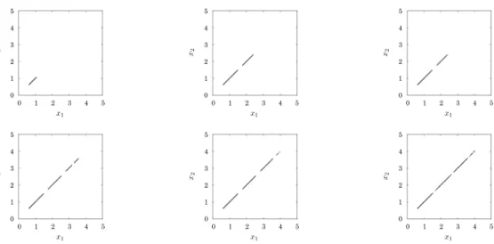
On the other hand, initial points in a laminar state, reaching a burst state within n (= 1, 2, 3, 5, 10, or 20) iterations, are depicted in Fig. 12. They show that the orbit tends to stay at smaller x

1

(= x

2

) values just before leaving the laminar state. They also implies that an exit from a laminar state to a burst state (around x = 1) is unstable in the direction perpendicular to the diagonal line.

4.3 Unstable Dimension Variability in Chaotic Itinerancy

Unstable dimension variability is characterized by the existence of cycles among invari- ant sets with different unstable directions

¹¹

. Tsuda (2009) conjectured that unstable dimension variability can be a key to understand the dynamics of chaotic itinerancy. In this subsection, we confirm that unstable dimension variability is observed in the two

11Homoclinic tangency and unstable dimension variability (hetero dimensional cycle) are thought to be typical structures which break hyperbolicity (Bonattiet al., 2005).

1 2 3 4 5 0

0 1 2 3 4 5

1 2 3 4 5

0 0 1 2 3 4 5

1 2 3 4 5

0 0 1 2 3 4 5

1 2 3 4 5

0 0 1 2 3 4 5

1 2 3 4 5

0 0 1 2 3 4 5

1 2 3 4 5

0 0 1 2 3 4 5

Fig. 12:

Routes from a laminar state to a burst state (ε=0.315). Among 10⁷initial points chosen from (x, y)∈(0,5)×(0,5), points reaching a burst state within 1, 2, 3 iterations (upper three, respectively) and 5, 10, 20 iterations (lower three, respectively) are plotted. It is implied that an exit from a laminar state to a burst state (aroundx= 1) is unstable in the direction perpendicular to the diagonal line.

dimensional map through identifying unstable periodic orbits with different unstable di- rections embedded in an attractor of on-off intermittency and confirming the existence of cycles among neighborhoods of the unstable periodic orbits.

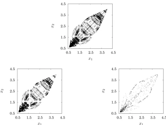
Unstable periodic orbits play an important role in characterizing chaotic systems including a system of chaos synchronization (Zhao et al., 2005). A number of unstable periodic orbits with periods up to 20 are depicted in Fig. 13. The upper graph shows all the points of the detected periodic orbits, which almost covers the chaotic attractor (Fig. 7 (right)). We distinguish the periodic orbits by the trajectory in the phase space.

A laminar periodic orbit is labeled if all points along the orbit stay in the laminar state, while a burst periodic orbit is labeled if at least one point on the orbit goes away from the laminar state. Among all the burst periodic orbits we classify the repeller (Fig. 13 (lower left)) and the saddle (Fig. 13 (lower right)) by the number of unstable directions. On the other hand, the distribution of x

₁

is investigated for laminar periodic orbits. Fig. 14 represents the distribution of saddles (left) and repellers (right)

¹²

. It is found that repellers tend to distribute around a repelling fixed point (x

₁

, x

₂

) = (1, 1).

Examples of time series of four types of periodic orbits are depicted in Fig. 15. The upper left corresponds to burst saddle (period 4), the upper right to burst repeller (period 6), the lower left to laminar saddle (period 10), and the lower right to laminar repeller (period 4). These imply that repellers tend to stay longer time around (x

₁

, x

₂

) = (1, 1).

In order to investigate how close a chaotic trajectory is to those four types of periodic orbits, we calculate distances between a chaotic trajectory and each periodic orbit in Fig. 16. The graphs show that a chaotic trajectory tends to approach to a point on each of four periodic orbits, implying the existence of an unstable dimension variability (heterodimensional cycle). That is, both saddles and repellers are embedded in both laminar and burst states and the connecting orbits among them exist.

12Here the bin width of the histogram is 0.1.

1.5 2.5 3.5 4.5 0.5

0.5 1.5 2.5 3.5 4.5

1.5 2.5 3.5 4.5 0.5

0.5 1.5 2.5 3.5 4.5

1.5 2.5 3.5 4.5 0.5

0.5 1.5 2.5 3.5 4.5

Fig. 13:

Distributions of unstable periodic orbits with periods up to 20 (upper). Distributions of burst repeller (lower left), burst saddle (lower right).

0.5 1 1.5 2 2.5 3 3.5 4 4.5 0

40 80 120 160

0 0 0.5 1 1.5 2 2.5 3 3.5 4 4.5

0 300 600 900 1200 1500

Fig. 14:

Histograms of a laminar saddle (lower left) and a laminar repeller (lower right). The former does not distribute around a fixed point (x1, x2) = (1,1), but the latter does.

5 Conclusion

In this study, we have robustly observed chaotic itinerancy and investigated its detailed structures in a model of regional business cycles coupled through producers’ adaptive behavior based on global information. The following results are obtained:

i ) The economy wanders among various regimes featuring different numbers of clus-

ters for particular constellations of parameters. Only a small coupling effect is

required for this phenomenon to occur. This implies that although all regions or

agents are economically homogeneous, the situation should not compel attention to

a “representative” region or agent; all must be considered simultaneously.

1 2 3 4 0

3

2

1 0.5 1.5 2.5

1 2 3 4

0 5 6

0.5 3

2

1 1.5 2.5 3.5

3

2

1 1.5 2.5 3.5 4

1 2 3 4

0 5 6 7 8 9 10

0.5

1 2 3 4

0 3

2

1 0.5 1.5 2.5

Fig. 15:

Examples of a burst saddle (period 4) (upper left), a burst repeller (period 6) (upper right), a laminar saddle (period 10) (lower left), and a laminar repeller (period 4) (lower right) (■: x1,

•

^{: x2).}

Fig. 16:

Distance between a chaotic orbitx(t) showing chaotic itinerancy and some pointxU P Oon each periodic orbit d(t) = minτ⩽tdist(x(τ), xU P O), where dist(·,·) denotes the Euclidean distance between two points (burst saddle in Fig. 15 (upper left), burst repeller (upper right), laminar saddle (lower left), laminar repeller (lower right)). All of them are shown to be passed by a chaotic itinerancy.

ii) When the producers emphasize the profit maximization and when they adjust their expectations slowly toward the average level announced by the government, the more likely the economy will exhibit chaotic itinerancy.

iii ) Behind chaotic itinerancy unstable dimension variability (heterodimensional cycle) may exist. This is identified by finding unstable periodic orbits with different number of unstable directions embedded in an attractor showing chaotic itinerancy, and cycles among them.

The dependency of occurrence of chaotic itinerancy on the system dimension remains an important issue for future work. The mechanism of the robustness of the phenomenon is to be clarified.

Acknowledgements

The authors would like to thank Professor Ichiro Tsuda for his helpful information about chaotic itinerancy. This work was partly supported by JSPS KAKENHI (Grant Number 26610034, 24653050, 23330086, 23740065) and by the Collaborative Research Program for Young Scientists of ACCMS and IIMC, Kyoto University.

References

Alexander, J. C., Yorke, J. A., and You, Z., 1992. Riddled Basins. International Journal of Bifurcation and Chaos 2, 795–813.

Antonakakis, N., 2012. Business Cycle Synchronization During US Recessions Since the Beginning of the 1870s. Economics Letters 117, 467–472.

Baxter, M., and Kouparitsas, M. A., 2005. Determinants of Business Cycle Comovement:

A Robust Analysis. Journal of Monetary Economics 52, 113–157.

Bonatti, C., D´ıaz L. J., and Viana, M., 2005. Dynamics beyond Uniform Hyperbolicity, Springer, Berlin.

Carlino, G. A. and DeFina, R., 1995. Regional Income Dynamics. Journal of Urban Economics 37, 88–106.

Carlino, G. A. and Sill, K., 2001. Regional Income Fluctuations: Common Trends and Common Cycles. Review of Economics and Statistics 83, 446–456.

Clark, T. E. and van Wincoop, E., 2001. Borderds and Business Cycles. Journal of International Economics 55, 59–85.

Fujisaka, H. and Yamada, T., 1983a. Stability Theory of Synchronized Motion in Coupled- Oscillator Systems. Progress of Theoretical Physics 69, 32–47.

Fujisaka, H. and Yamada, T., 1983b. Stability Theory of Synchronized Motion in Coupled- Oscillator Systems. II. Progress of Theoretical Physics 70, 1240–1249.

Glendinning, P., 2001. Milnor Attractors and Topological Attractors of a Piecewise Linear Map. Nonlinearity 14, 239–257.

Heagy, J. F., Platt, N., and Hammel, S. M., 1994. Characterization of On-Off Intermit-

tency. Physical Review E 49, 1140–1150.

Ikeda, K., Otsuka, K, and Matsumoto, K., 1989. Maxwell-Bloch Turbulence. Progress of Theoretical Physics. Supplements 99, 295–324.

Kaneko, K., 1990. Clustering, Coding, Switching, Hierarchical Ordering, and Control in Network of Chaotic Elements. Physica D 41, 137–172.

Kaneko, K., 2002. Dominance of Milnor Attractors in Globally Coupled Dynamical Systems with More than 7 ± 2 Degrees of Freedom. Physical Review E 66, 055201.

Kaneko, K., and Tsuda, I., 2000. Complex Systems: Chaos and Beyond. Springer, Berlin.

(English translation of the original Japanese version: Fukuzatsukei no Kaosu-teki Shinario, Asakura Publishing Co., Ltd., 1996).

Komuro, M., 2005. Shinban Kiso karano Rikigakukei (introduction to Dynamical Systems, newly-revised ed.). Saiensu-Sha Co., Ltd. Publishers, Tokyo. (In Japanese).

Kostelich, E. J., Kan, I, Grebogi, C., Ott, E., and Yorke, J. A., 1997. Unstable Dimension Variability: A Source of Nonhyperbolicity in Chaotic Systems. Physica D 109, 81–90.

Kouparitsas, M., and Nakajima, D. J., 2006. Are U.S. and Seventh District Business Cycles Alike? Federal Reserve Bank of Chicago. Economic Perspectives, 30, 41–60.

Kozlowski, P. J., 1995. Money and Interest Rates as Predictors of Regional Economic Activity. Review of Regional Studies 25 143–157.

Milnor, J., 1985. On the Concept of Attractor. Communications in Mathematical Physics 99, 177–195.

Onozaki, T., Sieg, G., and Yokoo, M., 2000. Complex Dynamics in a Cobweb Model with Adaptive Production Adjustment. Journal of Economic Behavior and Organization 41, 101–115.

Onozaki, T., Yanagita, T., Kaizoji, T., and Toyabe, K., 2007. Regional Business Cycle Synchronization through Expectations. Physica A 383, 102–107.

Pikovsky, A. S. and Grassberger, P., 1991. Symmetry Breaking Bifurcation for Coupled Chaotic Attractors. Journal of Physics A: Mathematical and Theoretical 24, 4587–

4597.

Rissman, E. R., 1999. Regional Employment Growth and the Business Cycle. Federal Reserve Bank of Chicago. Economic Perspectives 23, 21–39.

Selover, D. D., and Jensen, R. V., 1999. ‘Mode-Locking’ and International Business Cycle Transmission. Journal of Economic Dynamics and Control 23, 591–618.

Selover, D. D., Jensen, R. V., and Kroll, J., 2005. Mode-Locking and Regional Business Cycle Synchronization. Journal of Regional Science 45, 703–745.

S¨ ussmuth, B., 2003. Business Cycles in the Contemporary World. Physica-Verlag, Hei- delberg.

Tsuda, I., 1990. Possible Biological and Cognitive Functions of Neural Networks Prob- abilistically Driven by an Influence of Probabilistic Release of Synaptic Vesicles. In Proceedings of the 12th Annual International Conference, IEEE/EMBS, 1772–1773.

Tsuda, I., 2009. Hypotheses on the Functional Roles of Chaotic Transitory Dynamics.

Chaos 19, 015113.

Viana, R. L., and Grebogi, C., 2000. Unstable Dimension Variability and Synchronization

of Chaotic Systems. Physical Review E 62, 462–468.

Viana, R. L., and Grebogi, C., 2001. Riddled Basins and Unstable Dimension Vari- ability in Chaotic Systems with and without Symmetry. International Journal of Bifurcation and Chaos 11, 2689–2698.

Yasutomi, A., 2003. Itinerancy of Money. Chaos 13, 1148–1164.

Yetman, J., 2011. Exporting Recessions: International Links and the Business Cycle.

Economics Letters 110, 12–14.

Zhao, L., Lai, Y. C., and Shih, C. W., 2005. Transition to Intermittent Chaotic Synchro-

nization. Physical Review E 72, 036212.