Tide and Tidal Current in the Bali Strait,Indonesia

九州大学学術情報リポジトリ

Kyushu University Institutional Repository

Tide and Tidal Current in the Bali Strait, Indonesia

バリアンティ, デジー

https://doi.org/10.15017/1398415

出版情報：九州大学, 2013, 博士（理学）, 課程博士 バージョン：

権利関係：全文ファイル公表済

Tide and Tidal Current in the Bali Strait, Indonesia

DESSY BERLIANTY

July 2013

Tide and Tidal Current in the Bali Strait, Indonesia

A Dissertation

submitted for the degree of Doctor of Science

by

Dessy Berlianty  

Kyushu University

July 2013

ABSTRACT

The tide and tidal current, tide-induced residual current, and tidal front of the Bali Strait in Indonesia, are investigated, by using a 3-dimensional model called Coupled Hydrodynamical- Ecological for Regional and Shelf Seas (COHERENS). The elevation data at Pengambengan Station and the current velocity data at Bangsring Station, a narrow part in the Bali Strait provided by the Institute for Marine Research and Observation of Indonesia, are used to verify the model results. While the Bali Strait coastline and bottom depth data are obtained by smoothing a fine resolution bathymetry chart supplied by the Hydro-Oceanography Division of Indonesian Navy (DISHIDROS TNI-AL). Additionally, the image of sea surface temperature (SST) distribution from the satellite data, are employed to track the position of tidal front by comparing to the distribution of log ( H U

) value (where H is the water depth in meters and U the tidal current amplitude in ms

).

We started our study by running the model which was forced directly along the open boundary by four major tidal constituents (M

, S

, K

, and O

tides) from the global tidal elevation of ORI.96 model, which was developed by the Ocean Research Institute-University of Tokyo. The capability of our 3-d model for tidal simulation are confirmed in a good agreement with the observation data. Furthermore we find that the tidal type at Pengambengan Station can be classified into mixed, mainly semidiurnal. While the type of tidal wave in the narrow part of the Bali Strait is the standing wave, where the current direction goes northeastward at ebb tidal current and southwestward at flood tidal current.

Moreover co-amplitude chart of the Bali Strait shows that the tidal amplitude decreases gradually from the south of the Bali Strait toward the middle area of the strait and becomes to minimum in the northern part of the strait. Whereas the co-phase chart shows that the progressive wave are mainly coming from the Java Sea and the Indian Ocean.

The computed tide-induced residual current during the spring tide on May 16, 2010 in

the Bali Strait, shows a clockwise eddy in the shallow area at wide part of the strait and also a

small clockwise eddy in the south of the narrow strait.

The observed SST distribution near the narrow strait with the lower SST of 27 degrees, corresponds with small value of log ( H U

). And in the wide part of the strait, the log ( H U

) is larger and corresponds to higher SST of 29 degrees. Thus, we propose that the tidal front in the Bali Strait, generated between the stratification and vertical mixing area in the Bali Strait, is coincident along the line of log ( H U

) of 6.5.

PREFACE

This report presents the results of my study, supervised by Prof. Tetsuo Yanagi. The results has been published [Berlianty, D. and Yanagi, T., 2011, Tide and Tidal Current in the Bali Strait, Indonesia, Marine Research in Indonesia, Vol. 36, No. 2, pp. 25-36].

This study still continues and I wish I could present it in the near future with more comprehensive results that would be benefit.

The Institute for Marine Research and Observation under Ministry of Marine Affairs and Fisheries of Indonesia supports for the observation data (the sea level data were collected time- series in the framework of the Operational Oceanography Project, funded by the Indonesian Government).

MODIS (Moderate Resolution Imaging Spectroradiometer) Image Data used in this reports can be downloaded freely from OceanColor Homepage at: http://oceancolor.gsfc.nasa.gov/. And the MODIS image data with Hierarchical Data Format (HDF) were processed by using the Ferret program. Ferret is a product of NOAA's Pacific Marine Environmental Laboratory and used as well as for analysis and graphics in this reports. Information is available at http://ferret.pmel.noaa.gov/Ferret/.

Japanese Government Ministry of Education, Culture, Sports, Science and Technology

(MEXT) supports this study through a grant to the doctoral scholarship.

ACKNOWLEDGEMENTS

In the Name of Allah, the Beneficent, the Merciful. I praise Allah, the Almighty, on Whom ultimately we depend for sustenance and guidance. Indeed, without Allah Help and Will, nothing is accomplished.

I wish to express my deepest gratitude to my advisor, Professor Tetsuo YANAGI for his valuable advice and guidance of my study and research in Kyushu University. With his inspiration and enthusiasm, he provided ideas and guidance for my research and helped me in the writing of this thesis. It is my honour being his student.

Beside, I also would like to acknowledge Prof. Naoki Hirose, as Head of Ocean Modelling Group - Center for East Asian Ocean-Atmosphere Research, Kyushu University, for his genuine support, valuable advice, sincere comments and encouragement which help me a lot to finish this study, especially for my recent semester where I am as a member in his laboratory.

I would also like to express my gratitude to the official members of the dissertation committee, Prof. Kazuo Nakamura and Prof. Tomoharu Senju, their excellent advises and detailed review were very beneficial during the preparation of this thesis.

I am also indebted to Prof. Yutaka Yoshikawa, for his suggestions of learns at the earliest time of my study, and I owe my sincere gratitude to Prof. John Matthews for insightful discussions of MODIS data.

My gratitude also extends to my former advisor of Bandung Institute of Technology, Indonesia: Dr. Eng. Totok Suprijo and Dr. Eng. Nining Sari Ningsih, who constantly inspire and encourage in my study. I am also deeply indebted to my supervisor at the Institute for Marine Research and Observation, Indonesia: Berny A. Subki, Dipl.Oc. and Dr.rer.nat. Agus Setiawan, for their nice suggestions towards the planning of this study works.

I am also thankful to the numerous individuals who have directly or indirectly contributed to the completion of this study. I am particularly grateful to Ms. Harumi Fujii who was very carefully and patiently since the very first time of my application to study in Kyushu University.

Very valuable suggestions made by her have encouraged me in my study and life in Fukuoka.

Special thanks also are due to the staff of Student Support Center at the Kyushu University, and

particularly to Ms. Keiko James for their assistance in supporting any administration things. I also

thank all other members of the Marine Ecosystem, Ocean Dynamics, and Ocean Modelling Laboratory, and numerous friends, for always offering their care. To those who indirectly contributed in this study, their kindness means a lot to me. My heartful thanks to all of them.

Thank you very much.

I cannot finish without thanking my family. I warmly thank and appreciate my beloved

parents (Papa Mama) for their material and spiritual support in all aspects of my life. I also would

like to gratitude to my grandmother, my aunt, my late uncle, my mother-in-law and thankful to my

younger sister, younger brothers, and brother and sisters-in-law, for their endless love, prayers and

encouragement. And finally, I am particularly grateful to my husband for his enormous love, care,

support, prayer, and always cheer me up. I can just say thanks for everything and may Allah give

all the best in return.

The Holy Quran

The Holy Quran Surah Al-Baqara

Behold! In the creation of the heavens and the earth; in the alternation of the Night and the Day; in the sailing of the ships through the Ocean for the profit of mankind; in the rain which Allah sends down from the skies, and the life which He gives therewith to an earth that is dead; in the beasts of all kinds that He scatters through the earth; in the change of the winds, and the clouds which they trail like their slaves between the sky and the earth;― (here) indeed are signs for a people that are wise.

(The Holy Quran Surah Al-Baqara Verse 164)

CONTENTS

ABSTRACT  ... i

PREFACE ...  iii

ACKNOWLEDGEMENTS  ...  iv

CONTENTS  ...  vii

LIST OF FIGURES  ...  x

LIST OF TABLES  ...  xiv

LIST OF EQUATIONS ...  xv

CHAPTER I

 INTRODUCTION  ... 1

I.1

Background  ... 1

I.1.1

Tide and tidal current ... 3

I.1.2

Tide‐induced residual current and tidal front ... 4

I.2

The Objectives of Study  ... 7

I.3

Methodology of Study  ... 8

I.4

Structure  of Contents  ... 9

CHAPTER II

NUMERICAL MODEL  ...  11

II.1

COHERENS Description  ... 11

II.1.1

Basic hydrodynamic equations  ... 14

II.1.2

Sigma‐coordinate system ... 18

II.1.3

Turbulence schemes ... 20

II.1.4

Horizontal diffusion ... 21

II.1.5

Equation of state  ... 22

II.1.6

Boundary and initial conditions ... 22

II.1.7

Harmonic analysis ... 24

II.2 

Model Application to the Bali Strait  ... 26

II.2.1

Study area and model grid  ... 26

II.2.2

Initial model and open boundary ... 28

II.2.3

Output setting for harmonic analysis ... 29

CHAPTER III

RESULTS AND DISCUSSIONS  ... 30

III.1

Verification of Elevation and Current Velocity  ... 30

III.2 

Tide and Tidal Current  ... 37

III.3 

Propagation of Tidal Waves ... 43

III.4 

Residual Flow and Tidal Front ... 48

CHAPTER IV

SUMMARY AND CONCLUSION ... 56

IV.1

Summary ... 56

IV.2

Future Study  ... 59

BIBLIOGRAPHY ... 60

INDEX ... 65

LIST OF FIGURES

Figure 1

Location of the Bali Strait between Java Island and Bali Island, connecting the Java Sea 

and Indian Ocean  ... 1

Figure 2

Ikan Lemuru or Bali Sardinella (Whitehead, 1985) ... 2

Figure 3

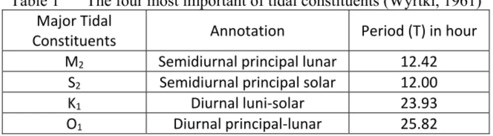
The fluctuation of lemuru production in the Bali Strait, 1974‐1994 (Merta, 1995) .... 2

Figure 4

The fish production in the Jembrana Regency (West Part of Bali), 2006‐2011 (Division  of Marine, Fisheries and Forestry of Jembrana Regency, Bali, 2012)  ... 2

Figure 5

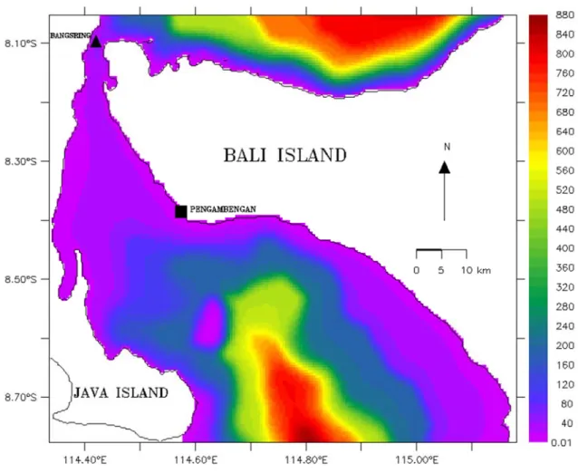
Bathymetric map of the Bali Strait, Indonesia. Filled‐colour show the depth in meters.  Black square shows the tide‐gauge station at Pengambengan and black triangle shows  the current observation station at Bangsring. ... 10

Figure 6

Conceptual diagram of the COHERENS model (Luyten P. , et al., 1999)  ... 13

Figure 7

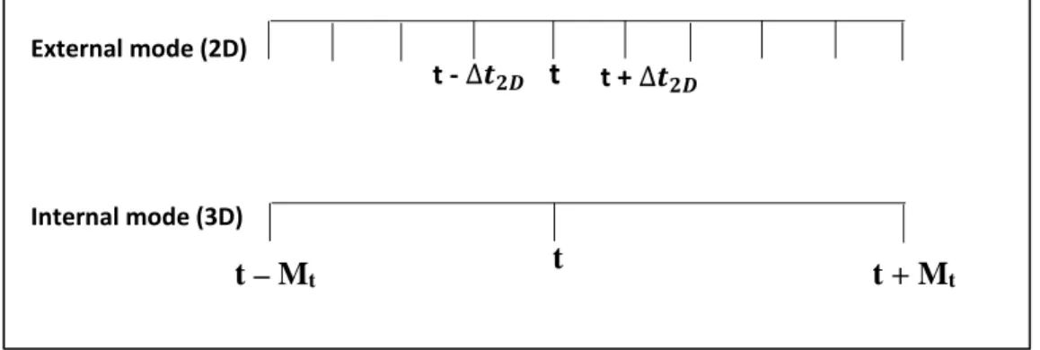
The mode splitting technique for time step  ... 14

Figure 8

The  σ ‐coordinate transformation in the vertical (Luyten et al., 1999) ... 19

Figure 9

The sigma‐coordinate system ...  20

Figure 10

Horizontal grid of domain model ... 27

Figure 11

Time series scheme of calculation period for 110 days ... 28

Figure 12

Simulation results at Pengambengan Station  for the period  of February 11

 to May  31

, 2010. Blue box shows the period of elevation verification and black box shows  the period of current  verification (upper).  Verification of elevation  (lower) between  the  observation  data  from  Institute  for  Marine  Research  and  Observation  (black‐

dotted line) and the simulation results (blue line) at Pengambengan for the period of  May 1

 to 31

, 2010.  ... 33

Figure 13

Verification of the current velocity component U in ms

 (x‐direction, eastward (+) ‐  westward (‐)) in (a), and component V in ms

 (y‐direction, northward (+) ‐ southward  (‐))  in  (b),  between  the  observation  data  at  Bangsring  Station  (full  line)  and  the 

simulation  results  (broken  line)  for  the  period  of  February  18

  to  19

,  2010. 

Simulation  results  of  elevation  (in  meters)  at  Bangsring  Station  for  the  period  of 

February 18

 to 19

, 2010 (c and d) are compared to the current velocity component. 

Point‐full line shows the elevation simulation, full line shows the current observation  and broken line shows the simulation results of tidal current. ... 36

Figure 14

The tidal amplitude spectrum of the observed (full line) and simulated result (broken  line) at  Pengambengan  Station,  with error swath  in  grey  colour  (upper  graph),  and  similarly  but  in  period  axis  (lower  graph)  for  the  tidal  amplitude  spectrum    of  the  observed (thick line) and simulated result (thin line), with error in broken line.  ... 38

Figure 15

The calculated depth averaged tidal current at the spring tide of the Bali Strait (May 

16

 2010), in ms

: (a) Tidal current at flood  water, (b) Tidal current at a  maximum 

flood (high water), (c) Tidal current at ebb water, and (d) Tidal current at a maximum  ebb (low water) . ... 40

Figure 16

The calculated depth averaged tidal current at the neap tide of the Bali Strait (May, 

22

  2010), in ms

: (a) Tidal current  at flood  water, (b) Tidal current at a maximum  flood (high water), (c) Tidal current at ebb water, and (d) Tidal current at a maximum  ebb (low water) . ...  42

Figure 17

The calculated co‐amplitude charts of four major constituents, colour filled contours  denote the magnitude of the co‐amplitude (in meters).  ... 45

Figure 18

The  calculated  co‐phase  charts  of  four  major  constituents,  colour  filled  contours  denote the co‐phase lines (°) referred to 8 h before GMT at 115°E.  ... 46

Figure 19

The  expanded  view  of  the  calculated  co‐phase  charts  of  four  major  constituents,  colour  filled  contours  denote  the  co‐phase  lines  (°)  referred  to  8  h  before  GMT  at  115°E.  ... 47

Figure 20

The calculated tide‐induced residual current (depth averaged) of the Bali Strait during  the spring tide on 2010 May 16

, in ms

. ... 49

Figure 21

Co‐range chart of M

, S

, K

, and O

 tidal current amplitude ... 52

Figure 22

The calculated contour line of log(H/U

) where H is the water depth in meters and   

the amplitude of tidal current in ms

, broken line show values less than 6.5, and full 

lines show values great than 6.5 ...  53

Figure 23

Aqua MODIS 8‐day composite Sea Surface Temperature (4 μ nighttime) – Level 3, with  time period from 17 May 2010 to 24 May 2010, showing the position of the tidal front  in  the Bali Strait.  The dark areas on the satellite  image  indicate warmer water.  The  light area in the north of the strait is due to the colder water. North is at the top of  the image and the grid size on the satellite image is 4 km

 resolution. ... 54

Figure 24

Fishing  Ground  Prediction  on  20  May  2010  (Institute  for  Marine  Research  and 

Observation, 2012) ... 55

LIST OF TABLES

Table 1

The four most important of tidal constituents (Wyrtki, 1961) ... 3

Table 2

Values of the parameters for the CFL‐criterion of the Bali Strait ... 15

Table 3

Switches for turbulence closure schemes in this study ... 21

Table 4

Values of the parameters in the equation state of the Bali Strait ... 22

Table 5

Frequencies for harmonic analysis  ... 25

Table 6

Summary  of  observation station  data used  in the  verification  period.  Locations  are  shown by black square and triangle in Figure 5. ... 30

Table 7

The tidal types range (Wyrtki, 1961)  ... 37

Table 8

The outline of the results ... 58

LIST OF EQUATIONS

Eq. (1) ... 15

Eq. (2) ... 15

Eq. (3) ... 15

Eq. (4) ... 16

Eq. (5) ... 16

Eq. (6) ... 17

Eq. (7) ... 17

Eq. (8) ... 17

Eq. (9) ... 17

Eq. (10) ... 18

Eq. (11) ... 21

Eq. (12) ... 21

Eq. (13) ... 22

Eq. (14) ... 22

Eq. (15) ... 23

Eq. (16) ... 25

Eq. (17) ... 31

Eq. (18) ... 31

Eq. (19) ... 34

Eq. (20) ... 34

Eq. (21) ... 34

Eq. (22) ... 34

Eq. (23) ... 35

Eq. (24) ... 35

Eq. (25) ... 37

CHAPTER I INTRODUCTION

I.1 Background

The Bali Strait, Indonesia, is a semi narrow passage located between Java Island and Bali Island (Figure 1), and connecting the Java Sea and the Indian Ocean in the northern part and the southern part of the strait, respectively. In addition to its importance of being the site of the regional port between both islands, the Bali Strait is also important for fisheries, where this strait is famous among fishermen especially in South Java and Bali region. In fact, one of the most important species amongst small pelagic in Indonesian Waters which concentrates in the Bali Strait, is ikan lemuru (Figure 2) or Bali Sardinella lemuru (Merta, 1995).

Figure 1 Location of the Bali Strait between Java Island and Bali Island, connecting the Java Sea and Indian Ocean

Along with an explanation by Salijo (1973) and Burhanuddin and Praseno (1982) also in

Merta (1995), they describes that the Bali Strait is so fertile that the biomass of the resource

becomes very high. As well as other researches by Hendiarti et al. (2005), Susanto and Marra

(2005) confirmed that the Bali Strait has rich nutrient with high biological and fisheries productivity. However as time goes, there are some threats such the extinction of the fishery potential in the Bali Strait. It can be seen from the graph of the fluctuation of lemuru production in the Bali Strait on period of 1974 to 1994 (Figure 3), where the fish catchment in 1986 was extremely low, that it has never occurred before (Merta, 1995). And from the graph in Figure 4 also confirms that the fish production in the Bali Strait seems like decreasing in the recent year.

The graph is taken from the report of Profile of Economy – Fisheries in Year 2012 of Jembrana Regency, Bali (Division of Marine, Fisheries and Forestry of Jembrana Regency, Bali, 2012).

Figure 2 Ikan Lemuru or Bali Sardinella (Whitehead, 1985)

Figure 3 The fluctuation of lemuru production in the Bali Strait,

1974-1994 (Merta, 1995) Figure 4 The fish production in the Jembrana Regency (West Part of Bali), 2006-2011 (Division of Marine, Fisheries and Forestry of Jembrana Regency, Bali, 2012)

Therefore, it needs a better understanding in order to know the behaviour phenomenon in the Bali Strait as explained above. Specifically it is necessary to first clarify the current field that could be used for the basic knowledge and supports primary productivity in order the future

17.6

27.8 26.5

44.5

23.3

12.6

2006 2007 2008 2009 2010 2011

Year

Fish Production (1000 ton)

investigation of the material transport in the coastal sea in the Bali Strait. The current field in the coastal sea mainly consists of the tidal current and the residual flow (Yanagi, 1999).

I.1.1 Tide and tidal current

At first, it is important basically to understand the characteristics of tide and tidal current field there because the transport of material such as nutrients and fish larvae is mainly governed by the tidal current (Yanagi, 1999). Various studies of the tidal characteristics from four major tidal constituents (Table 1) have been conducted in larger-domain of Indonesian Seas, such as Wyrtki (1961), Hatayama et al. (1996), and Ray et al. (2005).

Table 1 The four most important of tidal constituents (Wyrtki, 1961) Major Tidal 

Constituents  Annotation  Period (T) in hour  M2  Semidiurnal principal lunar  12.42 

S2  Semidiurnal principal solar  12.00 

K1  Diurnal luni‐solar  23.93 

O1  Diurnal principal‐lunar  25.82 

Despite not clearly shown, from the geographical distribution of the tidal types, Wyrtki (1961) showed that the Bali Strait has mixed, mainly semidiurnal tides, being an influence of the Indian Ocean. Wyrtki (1961) also explained that the tidal currents in Indonesian Seas are very strong and complex.

Studies by Ray et al. (2005) showed the cotidal charts of the largest semidiurnal tide M

and diurnal tide K

based on ten years of sea-level measurements from the Topex/Poseidon satellite

altimeter. In their results, the semidiurnal response is clearly dominated by the large tide from the

Indian Ocean, while the diurnal tide, in contrast to the semidiurnal, passes southwards and meets

the tide from the Indian Ocean with markedly increased amplitudes westward in the Java Sea. Note

also that their investigation merely concerns to general aspects in Indonesian Seas without a detailed explanation for the Bali Strait region.

Similarly, Hatayama et al. (1996) have also investigated the characteristics of tides and tidal currents in the Indonesian Seas, with particular emphasis on the predominant constituents, the barotropic M

and K

components. And they proposed that the tidal mixing could play an important role not only in the mixing process, but also in the transport process. In their study, there is also no detail explanation and investigation of the tidal characteristics in the Bali Strait.

Another study about oceanographic characteristics in the relation to the water fertility in the Bali Strait has been conducted by Priyono et al. (personal communication, 2013). They suspect the uniqueness of the water fertility and the abundance of lemuru are due to some factors, i.e.:

bathymetry, the semi-enclosed type of the strait, the tide and tidal current pattern, the limited of water mass from the freshwater discharge of the river, the chlorophyll-a and the essential nutrients.

However, they did not investigate and have no detail discussion about the descriptions of the tide- induced residual current and the tidal front.

I.1.2 Tide-induced residual current and tidal front

Hereafter, we also need to present the examination of the tide-induced residual flow and

tidal front which play very important roles in the dispersion matter in estuaries and also in the

primary productivity in the coastal sea. Yanagi (1976) explains that the tidal residual flow is

defined as the flow which is caused through the nonlinearity of tidal current in relation to the

boundary geometry and bottom topography and whose period of fluctuation is longer than that of

the tidal current. The circulation formed by the tidal residual flow is called the tide-induced

residual current, and it also plays a more important than tidal current for the dispersion of long- term material transport in the coastal area (Yanagi, 1974). Similarly Stacey et al. (2001) suggests that the residual circulation is critical to the management of the estuarine system. The health of an estuarine ecosystem is strongly dependent upon its residual circulation. While tidal currents may create large fluxes of nutrients and contaminants over the short timescale, it is the residual transport, which governs the residual exchange of material along the axis of the estuary.

Tides are one of main energy sources capable of generating vertical mixing in the ocean.

In shallow regions of the ocean (shelves, straits, and shoals), vertically mixed stationary zones with sharp frontal boundaries called tidal mixing fronts can be formed due to bottom friction. The zones of intense tidal mixing bounded by fronts are an important feature of the water structure of the shelf zone of the World Ocean (Zhabin & Dubina, 2012). Afterward, tidal front is a significant physical phenomenon in coastal waters. Tidal front plays an important role in the distribution of phytoplankton and zooplankton (Liu et al., 2003), also the coastal front plays important roles in the coastal ecosystem (Kiorboe et al., 1988), further the coastal front is well known as a good spawning ground for many fish species (Boucher et al., 1987).

The tidal front itself is generated at the transition zone between the stratified and vertically well-mixed regions (Yanagi, 1999). Further, the front itself is generated in a transition zone between cold water and warm oceanic water (Yanagi, et al., 1996). As well as explanation by Simpson (1981) that variations in the level of tidal stirring divide the shelf seas, during the summer regime, into well mixed and stratified zones separated by high SST gradient regions called fronts.

Since the satellite information is now one of the main tools for investigating the ocean (Zhabin &

Dubina, 2012), the front could be examined by using the discontinuity line between cooler of sea

surface temperature (SST) satellite image data and warmer SST. When the sea-surface heating is

dominant (warm period), a stratification develops where the tidal current is weak, and in the opposite condition (cold period), the water is vertically well-mixed where the tidal current is strong. Simpson and Hunter (1974) explained that the tidal front could appear in the transition zone between the stratified area due to the weak tidal current and the vertically well-mixed area due to the strong tidal current. They showed that the tidal fronts should lie along the line of the critical value of the parameter of log ( H U

) value, where H is the water depth in meters and U the tidal current amplitude in ms

. If the location of some given value of stratification parameter corresponds well with the frontal position of temperature, salinity, density, ocean current or chlorophyll-a, this critical value can be used to predict the mean tidal front’s position (Simpson &

Hunter, 1974).

However, as our best knowledge, no available discussion have been carried out on the occurrence and maintenance of the tide-induced residual current in the Bali Strait. There has been no study on the tidal front, which is also important in relation to the understanding of the accumulations of materials such as pollutants, nutrients and plankton along the frontal zones in the Bali Strait.

Eventhough various studies have been conducted to identify the tidal characteristics of the

Indonesian Seas, it still has limitation, for example, being unable to identify tide and tidal

characteristics in the narrow straits, e.g. the Bali Strait. Otherwise, it is also very difficult to

understand the tidal current field only by the limited results of direct current measurements in the

Bali Strait where cruise and fishing activity is very high. Furthermore, it is also impossible and

expensive to maintain the mooring system with current meters in the long term at many stations to

provide finer spatial distribution for the analysis. Inspite the data can be provided, they may not

be comparable due to difference of observation periods. There are several challenges and issues that need to be considered.

It is nearly impossible to clarify the current field using only field measurements because the coastal sea is too wide and deep to cover all the area by current meters. We have to carry out a numerical experiment in order to estimate the current field in the whole area of the coastal sea (Yanagi, 1999). Therefore under the limitation to obtain enough qualified observed data, in order to understand the physical phenomena for the basic knowledge and support primary productivity in the future in the Bali Strait, the numerical experiment could be a way to understand the structure of the physical and biochemical processes on a wide temporal and spatial scale (Yanagi, 1999).

I.2 The Objectives of Study

The overall aim of this study is to simulate the tide and tidal current in the Bali Strait effectively and efficiently by using a numerical modelling in order to more understand the physical phenomena in the strait. Within this aim, the specific objectives of this study to be reach are focused to the followings:



Investigation of the characteristics on the tide and tidal current in the Bali Strait, including the tidal wave and tidal propagation. This objective is addressed with data collected at Bangsring for tidal current and Pengambengan for tide (location shown in Figure 5).



Examination of the tide-induced residual current in the Bali Strait.



Furthermore, this study in particular analyzes the tidal front in the Bali Strait.

I.3 Methodology of Study

To achieve the objectives of this study, we employed the physical module of the 3-dimensional of COHERENS (a Coupled Hydrodynamical Ecological Model for Regional and Shelf Seas). This 3-d model was developed by Luyten et al. (1999), and it is based on vertical sigma-coordinate (see detail explanation in Chapter II of this thesis).

The elevation data at Pengambengan Station and the current velocity data at Bangsring Station, a narrow part in the Bali Strait (see Figure 5), were provided by the Institute for Marine Research and Observation, under the Ministry of Marine Affairs and Fisheries of Indonesia, and they are used to verify the model results. While the Bali Strait coastline and bottom depth data are obtained by smoothing a fine resolution bathymetry chart supplied by the Hydro-Oceanography Division of Indonesian Navy (DISHIDROS TNI-AL).

Meanwhile, to aim the examination of a tidal front, we analyze the value of parameter

where H is the water depth in meters and U the amplitude of the tidal current in ms

, as

suggestion by Simpson and Hunter (1974). Hereinafter, we seeks the corresponding of the log

value to detect fronts from the satellite image of sea surface temperature (SST). Additionally, the

image of sea surface temperature (SST) distribution from the satellite data, are employed to track

the position of tidal front by comparing to the distribution of log value. Thus we proposed the

generated position of mean tidal front based on the corresponding between the critical value of log

parameter with the frontal position of the SST image in the Bali Strait.

I.4 Structure of Contents

This thesis is structured as follows. At first, it begins by introducing and explaining the background and the motivation of this study which provides some previous researches in relation to this study. Hereafter, we will clarify the objectives of this study, and closed this chapter by the flowchart organization of this thesis.

Chapter 2 describes the COHERENS and numerical design that is used in the analysis.

Chapter 3 presents the validation between simulation and data, further followed by discussion of

our main results of the tide and tidal currents, the co-range and the co-phase to investigate the tidal

propagation, the tide-induced residual currents, and analyzing the fronts by parameter from

Simpson-Hunter (1974). It continues with the follow-up of SST fronts from the MODIS-Aqua

satellite image data, thus providing guidelines for comparison studies of tidal front. The last

chapter will summarizes the main results and propose the next step in the near future for the

continuation of this study.

Figure 5 Bathymetric map of the Bali Strait, Indonesia. Filled-colour show the depth in meters. Black square shows the tide-gauge station at Pengambengan and black triangle shows the current observation station at Bangsring.

CHAPTER II NUMERICAL MODEL

II.1 COHERENS Description

COHERENS is a three-dimensional multi-purpose numerical model for coastal and shelf seas (Luyten et al., 1999). The COHERENS model is available for the scientific community and can be considered as a good tool for better understanding of the physical character of coastal sea and the prediction of waste material spreading there. The code has been developed initially over the period 1990 to 1999 by a multinational group as part of the Marine Science and Technology Programme (MAST) projects of Processes in Regions of Fresh Water Influence (PROFILE), North Sea Model Advection Dispersion Study (NOMADS), and COHERENS, funded by the European Union (Luyten et al., 2002).

An important feature of COHERENS is that the time step and the horizontal and vertical resolution can be defined by the user in relation to the relevant time scale and the horizontal and vertical length scales which are imposed mainly by the physical forcing conditions. These are associated with processes on the mesoscale (wind, tides), the synoptic scale (frontal structures), the seasonal scale (thermocline formation, plankton blooms) and the global scale (climatic processes).

Other important advantages of the model are its transparency due to its modular structure and its flexibility because of the possibility of selecting different processes, specific schemes or different types of forcing for a particular application. The structure of COHERENS (Figure 6) consists of four main module as followings:



The physical module as a general module for solving advection-diffusion equations.



A biological module which deals with the dynamics of microplankton, detritus, dissolved inorganic nitrogen and oxygen.



An eulerian sediment module which deals with deposition and resuspension of inorganic as well as organic particles.



A component with both an eulerian and lagrangian transport model for contaminant distributions.

Hence we employed COHERENS to be used for the investigation of the physical characteristics in the Bali Strait. And due to the needs of our presents study, we focus to maximize the utilities in the physical module of COHERENS (orange box and line in Figure 6). And please make a note that the brief description on this sections is referred to Luyten et al. (1999) with adjusting the needed requirements to the present study in the Bali Strait.

  Figure 6 Conceptual diagram of the COHERENS model (Luyten P. , et al., 1999)

deposition resuspension

solar radiation meteorological

data

wind stress

tide and residual input

PHYSICAL MODEL

BIOLOGY

SEDIMENTS CONTAMINANTS

wave

bottom stress wave current interaction

surface elevation currents

density gradient

turbulence

advection diffusion module

fluff layer initial

concentration river and open

boundary input salinity temperature

meteorological data

heat fluxes

optical module

II.1.1 Basic hydrodynamic equations

The program allows to formulate the model equations either in Cartesian or spherical coordinates. The Cartesian computational grid has the advantage that the horizontal grid axes can be rotated arbitrarily in the horizontal plane, whereas the spherical computational grid takes account of the effects on the Earth’s curvature. Here we examine our model by applying the Cartesian coordinates.

The hydrodynamic part of the model uses the following basic equations:



the momentum equations,



the continuity equation,



the equation of temperature and salinity.

The equations of momentum and continuity are solved numerically using the mode- splitting technique (as illustrated in Figure 7). The method consists in solving the depth-integrated momentum and continuity equations for the external mode with small time step to satisfy the Courant-Friedrichs-Lewy (CFL) criterion, and also consists the 3-d momentum and scalar transport equations for the internal mode with a larger time step (Deleersnijder et al., as cited in Luyten et al. (1999).

Figure 7 The mode splitting technique for time step External mode (2D) 

Internal mode (3D) 

t ‐ ∆   t t + ∆  

t – Mt t t + Mt

The CFL criterion for the external mode is:

Δ 1

, Δ

2

  Eq. (1) 

where

is the minimum horizontal grid spacing, the maximum water depth,

, Ω 2π 86164

rad/s the rotation frequency of the earth,

The 3-d time step with a much longer time step Δ , i.e.:

Δ M Δ

Eq. (2)

where M values ranges from 10 to the following upper limit:

M Δ ⁄ Δ U

Eq. (3)

with U is a characteristic maximum value for the horizontal current. Thus, with assumption that U ~ 2 ms

and other value in Table 2, we found that the typical value of M ranges from 10 to 35.

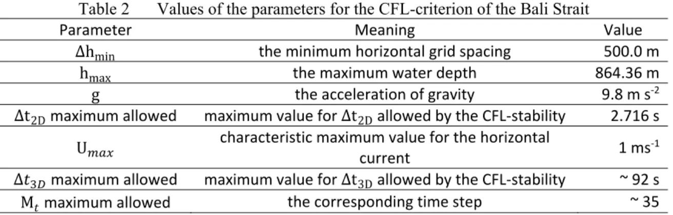
Table 2 Values of the parameters for the CFL-criterion of the Bali Strait

Parameter  Meaning  Value 

Δh_min  the minimum horizontal grid spacing  500.0 m

h_max  the maximum water depth  864.36 m

g  the acceleration of gravity  9.8 m s^‐2

Δt_2D maximum allowed   maximum value for Δt_2D allowed by the CFL‐stability   2.716 s

U   characteristic maximum value for the horizontal 

current  1 ms^‐1

Δ  maximum allowed  maximum value for Δt_3D allowed by the CFL‐stability  ~ 92 s

M

Based on those criterion, in present study we applied the time step for the 2-D Δ is set

to 2 seconds while the Δ is set to 60 seconds with the corresponding time step M is about of

30 (see Table 2 for detail calculation of this criterion).

Much effort has been made to implement suitable schemes for the advection of momentum and scalars, thus in this study we applying the TVD (Total Variation Diminishing) scheme to reduce the programming and computational overhead. This scheme is implemented with the symmetrical operator splitting method for time integration and can be considered as a useful tool for the simulation of frontal structures and areas with strong current gradients (Luyten et al, 1999).

This scheme using the superbee limiter as a weighting function between the upwind scheme and either the Lax-Wendroff scheme in the horizontal or the central scheme in the vertical. It has the advantage of combining the monotonicity of the upwind scheme with the second order accuracy of the Lax-Wendroff scheme.

The basic equations for the three-dimensional momentum equations are as followings:

1

Eq. (4)

1

Eq. (5)

Eq. (6)

and continuity equation: 

0

Eq. (7)

also the transport equations: 

1

Eq. (8) 

Eq. (9) 

where

are the current velocity components, T denotes the temperature, S the salinity, indicates time, for the Coriolis force, the acceleration of gravity, the pressure, and the vertical eddy viscosity and vertical diffusion coefficient, the horizontal diffusion coefficient for salinity and temperature, the density, a reference density, c

the specific heat of seawater at constant pressure and

solar irradiance.

Please note that in present study, we did not solve the transport equations due to the scope

of the study.

II.1.2 Sigma-coordinate system

In a sigma-coordinate system, the number of vertical levels in the water column is the same everywhere in the domain irrespective of the depth of the water column. This is achieved by transformation of the governing equations from z-coordinate to sigma-coordinate in the vertical as followings equation (Luyten et al., 1999):

    Eq. (10) 

so that sigma-coordinate varying between

8).

Notice that unlike the z-coordinate system, where the layer thicknesses are uniform in the

horizontal, it is the normalized thicknesses that are uniform in the sigma-coordinate system, while

the layer thicknesses vary widely from grid point to grid point. Also no grid point is wasted in the

vertical, unlike the z-coordinate model, where high resolution in deeper regions of an ocean basin

means inevitable loss of those grid points in shallower regions. Besides, the sigma-coordinate

enables the bottom (benthic) boundary layer to be better resolved everywhere in the domain. It is

easy to see that adequate resolution of the benthic layer everywhere in the domain can be achieved

in z-coordinates only with the use of a prohibitively large number of levels in the vertical.

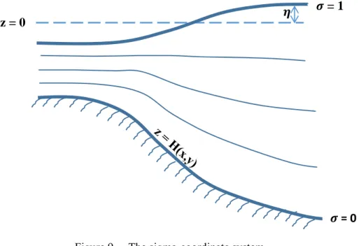
The

approximation of the surface and bottom baoundary conditions. In the Ζ-coordinate system, the layer thicknesses are uniform in the horizontal. Otherwise, in the σ-coordinate they are vary widely from grid point to grid point. Towards our study, we divided the vertical layer into 4 layer of uniform 0.25 sigma-interval (Figure 9).

y

y

Figure 9 The sigma-coordinate system

II.1.3 Turbulence schemes

One of the most intricate problems in oceanographic modelling is an adequate parameterisation of vertical exchange processes. In the COHERENS they are represented through the eddy coefficients and . The schemes of an adequate parameterisation of vertical exchange processes that implemented in the COHERENS have been developed and tested to represent the following physical process (Luyten et al., 1999):



turbulence generated by tidal friction in the bottom layer



wind-induced turbulence in the surface layer



enhancement of the bottom stress due to the interaction of waves and currents at the sea bottom



diurnal and seasonal cycles of heating and cooling, including the evolution of termoclines



shear-induced mixing at river fronts

 = 0  = 1  

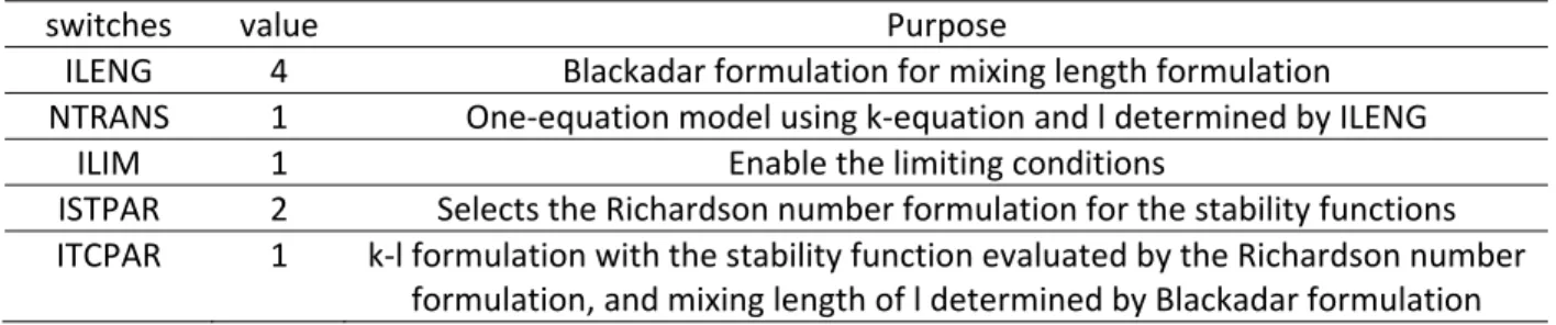
A large variety of turbulence parameterisation with a substantial range of complexity have been proposed and validated in the literature. In our study, we evaluated the vertical eddy viscosity and diffusion coefficient by using turbulence closure schemes (see Table 3 for the chosen value of each switch), and further detail could be found in Luyten et al. (1999).

Table 3 Switches for turbulence closure schemes in this study

switches  value  Purpose 

ILENG  4  Blackadar formulation for mixing length formulation  NTRANS  1  One‐equation model using k‐equation and l determined by ILENG 

ILIM  1  Enable the limiting conditions 

ISTPAR  2  Selects the Richardson number formulation for the stability functions  ITCPAR  1  k‐l formulation with the stability function evaluated by the Richardson number 

formulation, and mixing length of l determined by Blackadar formulation 

II.1.4 Horizontal diffusion

On COHERENS program, for the horizontal subgrid-scale processes not resolved by the model, are parameterised by the horizontal diffusion coefficients and . In this study, the horizontal diffusion coefficients are taken to be proportional to the horizontal grid spacings and the magnitude of the velocity deformation tensor in analogy with Smagorinsky’s parameterisation:

Δ Δ , Δ Δ

  Eq. (11) 

where

1

2

  Eq. (12) 

and

,

are the horizontal grid spacings (Luyten et al, 1999). In view of the uncertainty

concerning the values of the numerical coefficients and they are assumed to be equal,

which we adopted a value of 0.15.

II.1.5 Equation of state

An equation of state is required for the following reasons:



to evaluate the buoyancy in the equation of vertical hydrostatic equilibrium (Eq. (6),



to determine values for the thermal and salinity expansion coefficients and which are needed.

A linearised equation of state was chosen and taken of the following form:

1

  Eq. (13) 

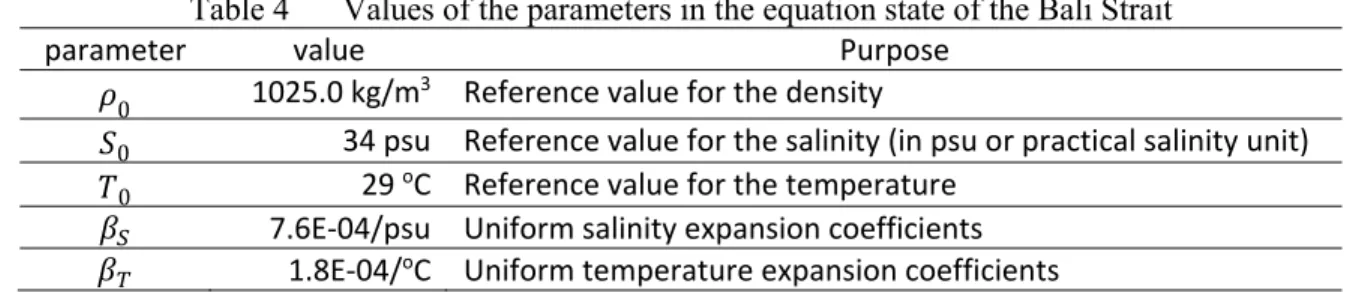
and , and are reference values for the density, salinity and temperature. Uniform values are used for coefficients and . Table 4 shows the values that used for the equation of state in our study.

Table 4 Values of the parameters in the equation state of the Bali Strait

parameter  value  Purpose 

0  1025.0 kg/m³   Reference value for the density 

0  34 psu  Reference value for the salinity (in psu or practical salinity unit) 

0  29 ^oC  Reference value for the temperature 

II.1.6 Boundary and initial conditions

Bottom boundary conditions

A slip boundary conditions for the Bali Strait study is applied for the horizontal current at the bottom which takes the form by using the quadratic friction law:

, ,

Eq. (14)

where the bottom velocities

are evaluated at the grid point nearest to the bottom. In the boundary layer approximation a vertically uniform shear stress is assumed yielding a logarithmic profile for the current. The quadratic bottom drag coefficient can then express as a function of the roughness length and the vertical grid spacing. This gives:

⁄

⁄

Eq. (15)

where

bottom cell. The value of which may vary in the horizontal directions, depend on the geometry and composition of the seabed. Here we use spatially uniform roughness length equal to 0.0035 m for the quadratic bottom drag coefficient.

Open sea and land boundary conditions

The model equations of COHERENS are solved on an Arakawa C-grid. Each grid cell has six lateral boundary faces. The boundary faces of a cell have one of the four following attributes:



Open sea boundary faces are always located along one of the four vertical planes (

and

which delineate the simulated area.



Interior boundaries are inside the domain and separate two wet cells.



Land boundaries are either situated along a boundary plane or in the interior domain where at least one of the two neighbouring cells must have a “dry” attribute.



River boundaries are either situated along one of the four domain boundaries or in the

interior domain at the interface between a “wet” and a “dry” cell. The difference with the

land boundaries is that the river boundaries are considered as impregnable walls whereas

the land boundaries constitute the “head” of a river where a specific boundary

condition (e.g. river discharge) is applied. For the present study, we did not use this type of

boundaries.

Coastal boundaries are considered as impregnable walls. This means that all currents, advective and diffusive fluxes are set to zero.

The open boundary conditions are based upon the form of a radiation condition derived using the method of Riemann characteristics. In the Bali Strait study, the open sea boundary conditions need to be supplied at southern and northern boundaries (see Figure 5). And four main tidal components M

, S

, K

, and O

are combined by using a global tide model ORITIDE (ORI.96;

the Japanese high-resolution regional ocean tide model) to provide time series of surface elevations (Matsumoto et al., 1995; 2000) along the open boundaries at northern and southern parts of the Bali strait (Figure 5).

ORI.96 ocean tide model was developed at Ocean Research Institute, University of Tokyo.

The ORI.96 model provides grid values of harmonic constants of pure ocean tide (0.5 x 0.5 degrees) and radial loading tide (1 x 1 degrees) for 8 major constituents (Matsumoto, et al., 1995).

Initial conditions

All currents are set to zero initially, and uniform values are taken for temperature and salinity, given by their reference values (see Table 4).

II.1.7 Harmonic analysis

In order to the analysis of the tide-induced residual current and investigate the log

parameter Simpson-Hunter in the Bali Strait, we apply an harmonic analysis that offers by the

program in COHERENS (Luyten et al., 1999). An harmonic expansion is written into the form as

followings:

, , ,

Eq. (16)

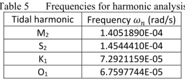
where is the residual, is the amplitudes, the phase is (with respect to the central time ), are a series of user-defined frequencies (see Table 5), and the number of harmonics in the analysis (4 tidal harmonics were used for this study).

Table 5 Frequencies for harmonic analysis Tidal harmonic  Frequency   (rad/s) 

M2  1.4051890E‐04  S2  1.4544410E‐04  K1  7.2921159E‐05  O1  6.7597744E‐05 

Other advantage by using COHERENS, the number and values of the frequencies that used in the harmonic analysis do not need to be the same as the ones appearing in the tidal forcing at the open boundaries. For example, if the model is forced with the M

tide only, higher order harmonics (M

, M

, …) are generated by the non-linearities of the model equations. These higher order terms can be investigated by applying an harmonic analysis in COHERENS.

Alternatively, the method can be used to analyze the evolution of a M

tide during a spring- neaps cycle, e.g. by forcing the model with a M

and S

tide and performing the analysis with only the M

frequency at different times t=t

, t

+T, … (Luyten, et al., 1999).

In present study, the model in the Bali Strait was forced by 4 major of M

, S

, K

, and O

tides, as similar as the evolution for the harmonic analysis investigation.

II.2 Model Application to the Bali Strait

II.2.1 Study area and model grid

The Bali Strait of Indonesia is located between 8.0546379

S – 8.7746868

S of latitude and 114.3389435

E – 115.1776276

E of longitude, Figure 5 shows the topography of the Bali Strait, where the bathymetric data was obtained from Hydro-Oceanography Division – Indonesian Navy (DISHIDROS TNI AL), Bathymetric Map No. 290 with scale 1:200,000, edition of March 2006. Bathymetry of the Bali Strait is shallow in the narrow part with average depths of about 50 m, and deep at northern and southern part with depths range of about 100 – 800 m.

The description model setup for the Bali Strait is explained below. The model equations

which explained above are solved on Cartesian grid. The computational domain is the Bali Strait

with the northern boundary taken at 8° 3' 16.6968" S and the southern boundary taken at 8° 46'

28.8732" S (Figure 10).

Figure 10 Horizontal grid of domain model

The horizontal grid is in the Cartesian coordinate system. This study area is horizontally represented by a rectangular computational domain discretized with regular Arakawa C-grid system. The computational grid has a resolution of 0.2703’ in both latitude and longitude corresponding to a grid spacing of 0.5 km or one cell grid is 500 m x 500 m, contained 186 x 160 grid points. The external time step of barotropic equations is 2 seconds to satisfy the Courant- Friedrichs-Lewy (CFL) criterion and 60 seconds for the internal time step.

Without considering temperature, ecology, thermodynamics and sediment modul in

COHERENS, the model operates also without the influences of the wind velocity and vertical

stratification of temperature and salinity. Thus, the vertical water column is divided into 4 layers

in a uniform 0.25 interval and the grid is vertically irregular as the result of σ–coordinate transformation (Figure 8).

II.2.2 Initial model and open boundary

The model of this study was initialized with zero elevation and velocity throughout the domain. Open boundaries of the model area are at the northern and southern open boundaries.

Along the open boundaries at northern and southern parts of the Bali Strait, the sea surface elevation are prescribed by using hourly time series prediction from the ocean global tide model ORITIDE. The time series of surface elevation taken based on the combination of four main tidal components M

, S

, K

, and O

.

The simulation was run for 110 days, starts from the 11

of February 2010 00.00 local time (+08 GMT) and ends at the 1

of June 2010 00.00 local time (+08 GMT). The simulation period is to cover the periods of tidal current and tide observations, on 18

to 19

February 2010 and 1

to 31

May 2010, respectively (Figure 11).

Figure 11 Time series scheme of calculation period for 110 days

Start 

February  11^th 2010 

End 

May  31^th 2010  Tide observations 

1 – 31 May 2010  Tidal current observations 

18 – 19 February 2010 

II.2.3 Output setting for harmonic analysis

In the interest of this study to understand the physical phenomenon such tidal

characteristics in the Bali Strait, we’ve only utilized the application of the physics model as one of

the main program components of COHERENS (instead of biological model, sediment model, and

contaminant model). There is no special treatment in order to attain convergence of the numerical

solution since it was found by Luyten et al. (1999) that the model reaches good numerical

convergence. On this study, the special output was to make use of the program’s utility of

COHERENS to perform an harmonic analysis (by activated the subroutine of defanal.f) where the

tide-induced residual flow, amplitude and phase are obtained by the program of harmonic analysis

for the period of 15

– 17

of May 2010 (~ 6 tidal cycles) to examine its correspondence to the

satellite data in the spring tide.

CHAPTER III RESULTS AND DISCUSSIONS

III.1 Verification of Elevation and Current Velocity

To test the capability of our 3-D model for tidal simulation, we ran the model forced directly by the global tidal elevation along the open boundary and verified to the observation data (Table 6).

In this study, the sea-level data at 1-hour intervals were obtained from the original tide- gauge time series at Pengambengan Station (marked with black square on Figure 5), which belongs to the Institute for Marine Research and Observation, under the Ministry of Marine Affairs and Fisheries of Indonesia, whereas the current velocity data were collected at Bangsring Station (marked with black triangle on Figure 5).

Table 6 Summary of observation station data used in the verification period. Locations are shown by black square and triangle in Figure 5.

Station  Position  Period of 

Observation 

Type of Observation  Source 

Pengambengan  114.574684 ^oE,  8.385226 ^oS 

1 – 31 May  2010 

Hourly sea level data 

Institute for  Marine Research 

and Observation  Bangsring  114.420548 ^oE, 

8.086338 ^oS 

18 – 19  February 2010 

20 minutes interval  of current velocity 

The current velocity observation depth is 20 meters and the data time interval is 20 minutes of vertically averaged profile records which was measured with an Acoustic Doppler Current Profiler (ADCP) of SonTek Argonaut propeller.

Simulation results of elevation at Pengambengan Station for the period of February 11

to

May 31

2010 are shown in Figure 12 (upper) where blue box shows the period of tidal verification

and black box shows the period of current verification.

Verification of elevation is shown in Figure 12 (lower) to compare the observation data from Institute for Marine Research and Observation (black-dotted line) and our simulation results (blue line) at Pengambengan for the period of May 1

to 31

2010.

To analyze whether our simulated elevations are in a good agreement with the observed data, we were assessing two methods of statistics, that is: the Root Mean Square Error (RMSE) and r-squared (r

). Both methods are based on two sums of squares: Sum of Squares Total and Sum of Squares Error (Grace-Martin, 2005).

The RMSE is the square root of the variance of the residuals. It indicates the absolute fit of the model to the data (how close the observed data points to the model’s predicted value. Lower values of RMSE indicate better fit. The general equation for root mean square error (RMSE) is:

∑

Eq. (17)

where is the total number of estimated values to be evaluated, is the calculated value (calculated elevation), and is the known “true” value (elevation data).

Otherwise, the r

has the useful property that its scale is intuitive; it ranges from zero to one, with zero indicating that the proposed model does not improve prediction over the mean model and one indicating perfect condition. The formula to calculate the r

are as followings:

∑

  Eq. (18) 

where is the total number of estimated values to be evaluated, is the data value, is the mean,

and is the model value (calculated elevation).

Based on both methods as explanation above, we found that the RMSE is 0.29 meters and

the Root-squared (r

) is 0.813. It indicates that our elevation model adequately fits to the data.

      33

Figure 12 Simulation results at Pengambengan Station for the period of February 11^th to May 31^th, 2010. Blue box shows the period of elevation verification and black box shows the period of current verification (upper). Verification of elevation (lower) between the observation data from Institute for Marine Research and Observation (black-dotted line) and the simulation results (blue line) at Pengambengan for the period of May 1^st to 31^st, 2010.

The calculated current velocities at Bangsring Station for the period of February 18

to 19

2010 are shown in Figure 13 and are compared to the observation of current velocity. The current velocity components of x (U; East-West direction) and y direction (V; North-South direction) indicate that simulation results are a little larger than the observation data (Figure 13(a) and Figure 13(b)). We suppose the difference between simulation and current data is due to the estimation of the effect of the bottom friction which does not reproduce adequately the nonlinear interaction of the extremely strong tidal currents with the bottom topography.

Furthermore, Figure 13(c) and (d) shows that there is a phase-lag of about three hours between the calculated elevation and the current velocity at Bangsring Station (the narrow part of the strait, see location in Figure 5). It could be explained as in Yanagi (1999) by the vertically integrated equations of motion and continuity under the assumption of linear motion and non-viscous fluid in 1-dimension of the bay, as

∂u

∂t ‐g∂η

∂x

Eq. (19)

where g the acceleration of gravity, η the elevation, and

∂η

∂t h∂u

∂x 0

Eq. (20)

with a uniform depth h and length l. Thus shortly, by assuming that

u U₀sin σt

at x l Eq. (21)

and

u 0 at x 0

Eq. (22)

where

the tidal current amplitude, hereafter the solutions are obtained as

η x,t U₀ h g

cos kx

sin kl cos σt

Eq. (23)

and

u x,t U₀sin kx

sin kl sin σt

Eq. (24)

where k shows the wave number (k 2π/L), and L the wavelength of the tidal wave.

The solutions show that the phase of sea level variation and current variation differ by π/2 (3 hours) and it indicates that the type of tidal wave in the narrow part of the Bali Strait is a standing wave, where the current direction goes northeastward at ebb tide and southwestward at flood tide. Therefore, there is a little phase difference of tide and tidal current in the Bali Strait and the high water, low water, flood and ebb happen at nearly the same time.

In other words, the tidal wave behaves and forms a standing wave in the narrow part of the

Bali Strait (i.e. Bangsring station area), because both incident tidal waves southward propagation

coming from the Java Sea and northward propagation coming from the Indian Ocean superpose

there.

(-)) in (a), and component V in ms^-1 (y-direction, northward (+) - southward (-)) in (b), between the observation data at Bangsring Station (full line) and the simulation results (broken line) for the period of February 18^th to 19^th, 2010. Simulation results of elevation (in meters) at Bangsring Station for the period of February 18^th to 19^th, 2010 (c and d) are compared to the current velocity component. Point-full line shows the elevation simulation, full line shows the current observation and broken line shows the simulation results of tidal current.