A Simple Method for Calibrating Uniform Linear Array
Xiang Cao
#∗1, Jingmin Xin
#, Yoshifumi Nishio
∗2, Nanning Zheng
#, Akira Sano
†3#
Institute of Artificial Intelligence and Robotics, Xi’an Jiaotong University Xi’an 710049, China
∗
Department of Electrical and Electronic Engineering, The University of Tokushima Tokushima 770-8506, Japan
†
Department of System Design Engineering, Keio University Yokohama 223-8522, Japan
Abstract—In this paper, a simple auto-calibration method
is presented for estimating spatial signature with uncalibrated uniform linear array. The proposed method is an extension of Esprit-like method and also extracts two subarrays to construct an estimator. The difference is that one element of array can be used several times in one subarray. A closed-form solution is obtained. Simulation results indicate that our algorithm performs better than Esprit-like. Furthermore, the simple algorithm could be used to initialize the multidimensional search method in [1].
I. I
NTRODUCTIONIn sensor array signal processing, many high-resolution methods such as ESPRIT [2] have been advanced for esti- mation of unknown parameters embedded in an array output model. It is a natural motivation of array calibration, since the performance of these methods will degrade dramatically when the ideal array model is damaged by some unknown errors (e.g., mutual coupling and sensor position uncertainties).
Two parametric errors (i.e., statistical and deterministic) were usually used to extend the ideal array model. This paper only focus on the deterministic unknown gain and phase errors.
The term deterministic here implies that the unknown error at each of elements of array is a stable constant during the period of observation.
Several so-called autocalibration approaches have been de- veloped in literature. Here, the autocalibration indicates that array calibration may be accomplished without employing any dummy elements or transmitters at known direction. In [3], an iterative eigenstructure-based technique of estimating Direction of Arrival (DOA) in the presence of unknown gain and phase errors is presented and it can apply to arbitrary array geometries except Uniform Linear Array (ULA). For ULA, a phase ambiguity exists between the diagonal error matrix and the ideal array steering matrix (see [4] and [5]).
Thus, it is impossible to estimate DOA and gain and phase errors simultaneously for ULA from array output. A Hermitian Toeplitz structure of ULA output covariance matrix in the
absence of gain and phase errors is exploited in [6] and [7].
This method takes advantage of the elements equivalence at every diagonal line to form two equations for estimation of gain and phase errors. The main drawback of the approach is that the Toeplitz matrix assumption is only established under infinite sampling condition. It means that if the number of snapshots is fixed, the performance of the algorithm does not improve after increasing the signal-to-noise ratio (SNR) to a certain point. In addition, the ESPRIT method also can be extended to the case. The idea firstly emerged from [8], and is applied for estimating spatial signature in [9] and [5]. The Esprit-like method (see [5]) constructs an estimator based on the maximum overlapping two subarrays. However, it has been pointed out in [10] that any two subarrays configuration may be inherently suboptimal. In [1], we proposed a multidimen- sional search procedure to estimate spatial signature. Unlike Esprit-like method, the algorithm fully exploits the multiple invariances inherent ULA even though the array model errors exist.
In this paper, we consider the spatial signature estimation problem with ULA in the presence of unknown gain and phase errors. The practicality of spatial signature can be found in [9] and [5]. The sensor gain and phase errors are different from mutual coupling among elements of array and it can not be affected by other sensors. Furthermore, the ideal steering matrix of ULA has a Vandermonde structure. Both of them provide the possibility of selecting subarrays from uncalibrated array like ESPRIT. In practice, A simple eigenstructure-based algorithm is presented. Two subarrays are firstly extracted from ULA to construct an estimator. The difference with Esprit-like method is that one element of ULA can be used several times in one subarray. Our method firstly estimates the rotational DOAs (not absolute DOAs) and error parameters, then obtains the estimation of spatial signature.
- 134 -
IEEE Workshop on Nonlinear Circuit Networks December 14-15, 2012
II. DATA MODEL
A uniform linear array with M sensors received narrowband signals from p far-field sources and the vector response y ∈ C
M×1of the array at time t can be expressed as
y(t) = Γ(γ)A(θ)s(t) + n(t), (1) where s(t) ∈ C
p×1is the vector of incident signals at time t, n(t) ∈ C
M×1is the vector of additive noises, the steering matrix A(θ) = [
a(θ
1) a(θ
2) · · · a(θ
p) ]
is the ideal array response, and
a(θ) = [
1 e
j2πλdsin(θ)· · · e
j2πλ(M−1)dsin(θ)]
T. (2) Here, operator ( · )
Tstands for transpose, θ
1, θ
2, · · · , θ
pare the directions-of-arrival of signals, d and λ represent the distance between two consecutive sensors and the identical wavelength for all signals, respectively. The diagonal matrix Γ(γ) is given by
Γ(γ) = diag [
γ
1γ
1· · · γ
M] , (3) and | γ
i| > 0 denotes the deterministic unknown gain and phase error of sensor i. The vector γ is constructed out of the diagonal elements of matrix Γ. For simplicity, Γ(γ) and Γ denote the same matrix.
Two assumptions need to be made. Firstly, signal s(t) is a temporally complex white Gaussian random vector with mean zero and its covariance matrix Rss has full rank p (assuming no correlate signals). Secondly, noise n(t) is a temporally and spatially complex white Gaussian random vector with mean zero and uncorrelated with incident signals. Then, the so-called signal subspace E
sand noise subspace E
ncan be easily obtained from the eigenvalue decomposition of array output covariance matrix
R = E { y(t)y
H(t) } =
∑
M i=1λ
ie
ie
Hi, (4) where E {·} and ( · )
Hdenote the statistical expectation and the complex conjugate transpose, respectively. The eigenvalues are ordered such as λ
1≥ λ
2≥ · · · ≥ λ
p> λ
p+1=
· · · = λ
M. The corresponding signal subspace E
sand noise subspace E
nare given by E
s= [
e
1· · · e
p] and E
n= [
e
p+1· · · e
M] .
The focus of this paper is the estimation of Spatial Signature matrix H = Γ(γ)A(θ) (instead of absolute DOAs) from the N snapshots of the array output. One ambiguity for this problem may be observed between the unknown signal vector s(t) and H (i.e., Hs(t) = αH · (
α1s(t)) for an unknown non-zero scaling α). A reasonable constraint for solving this scaling ambiguity is to let the first element of diagonal matrix Γ(γ) be equal to one.
III. ESTIMATION ALGORITHM
A simple subspace approach is presented for estimating spatial signature matrix H in this section. The Vandermonde structure of the ideal array steering matrix A permits optimally
exploiting invariance for ULA even though the gain and phase of the sensor have not been calibrated.
Since the one-to-one correspondence between rows in H and elements of array, extracting a subarray from array is equivalent to picking up rows of matrix H. Define a selection matrix J
m×(M−ε)consisting of zeros and ones. Only one element at every row is equal to one and it corresponds to the selected sensor of the array. However, the number of one each column in J
m×(M−ε)indicates the number of repetitions of selected element in subarray.
Then, the spatial signature matrix H can be partitioned into two subarrays
J ΓA =
[ Γ
xA
xΓ
yA
xΦ
ε]
, (5)
where J =
[ J
1J
2]
=
[ J
m×(M−ε)0
m×ε0
m×εJ
m×(M−ε)]
, (6)
and εd denotes the distance between two subarrays. Γ
x, Γ
yand A
xmay be calculated by the following equations:
Γ
x= diag { J
1γ } , Γ
x= diag { J
2γ } , A
x= J
1A. (7) The displacement diagonal matrix Φ is given by
Φ = diag [
e
j2πλdsin(θ1)· · · e
j2πλdsin(θp)]
. (8)
Here, we give an example of selection matrix. Consider a ULA with six elements, a possible selection matrix J
9×5may be expressed as
J
9×5=
1 0 0 0 0 0 1 0 0 0 0 0 1 0 0 0 1 0 0 0 0 0 1 0 0 0 0 0 1 0 0 0 1 0 0 0 0 0 1 0 0 0 0 0 1
. (9)
The determinant of the matrix Γ(γ) is given by det(Γ(γ)) =
∏
M i=1γ
i̸ = 0, (10)
then the rank of the matrix H is p, i.e., Rank(ΓA) = p.
It is clear that the matrix ΓA spans the same space as the signal subspace E
s. The relationship implies that there exists a nonsingular p × p matrix T satisfying
J E
s= [ E
xE
y]
= J ΓAT . (11)
Combining equation (5) and (11) leads to
E
x= Γ
xA
xT , E
y= Γ
yA
xΦT ¯ (12) where diagonal matrix Φ ¯ = Φ
ε. Eliminating A
xyields to
Γ(¯ ¯ γ)E
y= E
xΨ (13)
- 135 -
where the m × m diagonal matrix Γ(¯ ¯ γ) = Γ
−y1Γ
xand Ψ = T
−1ΦT. The vector ¯ γ ¯ is constructed from the diagonal elements of matrix
Similar to Esprit-like method in [5], Γ(¯ ¯ γ) and Ψ can be estimated from the least squares problem as follow
ˆ ¯
Γ, Ψ ˆ = arg min Γ
¯,Ψ
Γ(¯ ¯ γ)E
y− E
xΨ
2F
. (14)
The solution for Ψ is give by Ψ ˆ =
( E
HxE
x)
−1E
HxΓ(¯ ¯ γ)E
y. (15) Substituting back to (14) and after some manipulation, the least squares problem becomes
ˆ ¯
γ = arg min γ
¯γ ¯
H[
Π
⊥E
x⊙ ( E
yE
Hy)
T]
¯
γ, (16)
where Π
⊥E
x= I − E
x( E
HxE
x)
−1E
Hx. From above equa- tion, an estimate of vector γ ¯ may be obtained from the eigenvector associated with the smallest eigenvalue of the matrix Π
⊥E
x⊙ (
E
yE
Hy)
T. Here we note that constraint may be added to matrix Ψ and some discussions about this question can be found in [5]. Consider the example of (9), the two diagonal matrices Γ
xand Γ
ymay be expressed as
Γ
x= diag { 1, γ
2, γ
3, γ
2, γ
3, γ
4, γ
3, γ
4, γ
5} (17) and
Γ
y= diag { γ
2, γ
3, γ
4, γ
3, γ
4, γ
5, γ
4, γ
5, γ
6} . (18) Recall Γ(¯ ¯ γ) = Γ
−y1Γ
x, we can see that once an estimate of vector γ ¯ is obtained from (16), it is convenient to computer the elements of vector γ. Furthermore, the matrix Ψ can be obtained by Substituting the matrix Γ(¯ ¯ γ) reconstructed from ˆ ¯
γ back to (15).
The proposed algorithm now is briefly outlined below.
1) Estimate the signal subspace E ˆ
sfrom the eigende- composition of the sample covariance matrix R ˆ =
1 N
∑
Nn=1
y(n)y
H(n), where N is the finite number of snapshots.
2) Calculate E
xand E
yaccording to (11), then determine an estimate of vector γ ¯ from (16).
3) Calculate the matrix Ψ according to (15), then extract the rotational DOA θ. ˆ
4) Construct matrix Γ(ˆ γ) and A(ˆ θ), then spatial signature matrix is estimated as H ˆ = Γ(ˆ γ)A(ˆ θ).
IV. EXPERIMENT
In this section, computer simulation were conducted for evaluating the performance of the proposed algorithm. The results of the methods in [5] and [1] are also included. In this scenario, a ULA of 9 elements with half of wavelength element spacing is used. In [1], the ULA is divided into 5 subarrays and the ith subarray is selected by matrix J ˜
i=
−100 −8 −6 −4 −2 0 2 4 6 8 10
0.1 0.2 0.3 0.4 0.5 0.6 0.7 0.8
SNR(dB)
RMSE
Esprit−like
Method2 initialized by method1 Method1
Method2 initialized by Esprit−like
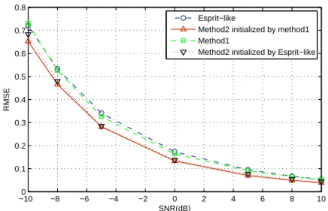
Fig. 1. RMSE of the spatial signature matrixH estimation versus SNR.
The number of snapshots N=600
[0
5×(i−1), I
5×5, 0
5×(5−i)], i = 1, · · · , 5. However, the two subarrays in this paper are selected by matrices
J
1= [
J ˜
T1J ˜
T2J ˜
T3J ˜
T4]
T(19) and
J
2= [
J ˜
T2J ˜
T3J ˜
T4J ˜
T5]
T. (20)
The deterministic gain and phase errors are given by 1, 1.10e
j10◦, 0.90e
−j5◦, 1.25e
j20◦, 0.80e
−j9◦, 0.96e
j15◦, 1.18e
−j23◦, 0.88e
−j2◦and 0.85e
j4◦. Two equal-power un- correlated signals located at 25
◦and 45
◦are considered and the SNR per element for each source is defined by SNR = 10 log
10(σ
s2/σ
n2), where σ
s2and σ
n2, respectively, denote the power of incident signal and that of additive noise at each sensor. RMSE is used as the performance measure and defined by
RMSE = 1 K
∑
K i=1√ H ˆ
i− H
i2
F
, (21)
where K is the number of trials, H ˆ
iand H
iare the estimated spatial signature and the true one at the ith experiment. A total of 500 trials were performed for each simulation scenario.
In Figure 1, method1 and method2 denote the proposed algorithm in this paper and in [1], respectively. Note that method1 could be used to initialize method2. The simulation result shows that our method performs better than Esprit-like even at low SNR. It means that the maximum overlapping subarray is not the optimal choice in the presence of unknown sensor gain and phase response. In other words, fully exploit- ing invariance inherent array should be taken into account. In addition, the behaviour of the iterative scheme (method2) has been improved significantly when the initial parameter values were provided by our method.
V. C
ONCLUSIONA simple eigenstructure-based algorithm is presented for spatial signature estimation for ULA with unknown gain/phase errors. Our method fully excavates the invariance of the ULA instead of simply using maximum overlapping subarray in
- 136 -
Esprit-like in [5] and give a closed-form solution. How to select subarrays from ULA, making the algorithm lead to optimal parameter estimation, is not addressed in this paper.
Some pragmatic discussion about this question can be found in [10].
A
CKNOWLEDGMENTThis work was supported in part by the National Nature Science Foundation of China under Grant 61172162.
R
EFERENCES[1] X. Cao, J. Xin, Y. Nishio, N. Zheng, and A. Sano, ”A method for spatial signature estimation with uncalibrated uniform linear array,”
Proc. SSPD2012 (in press).
[2] R. Roy and T. Kailath, “ESPRIT-estimation of signal parameters via rotational invariance techniques,” IEEE Trans. Acoust.,Speech, Signal Process., vol. 37, no. 7, pp. 984-995, 1989.
[3] A. J. Weiss and B. Friedlander, “Eigenstructure methods for direction finding with sensor gain and phase uncertainties,” Circuits Syst. Signal Process., vol. 9, no. 3, pp. 272-300, 1990.
[4] J. Pierre and M. Kaveh, “Experimental performance of calibration and direction-finding algorithms,” Proc. ICASSP’91, PP. 1365-1368, 1991.
[5] D. Ast´ely, A. Swindlehurst, and B. Ottersten, “Spatial signature estima- tion for uniform linear arrays with unknown receive gains and phases,”
IEEE Trans. Signal Prosess., vol. 47, no. 8, pp. 2128-2138, 1999.
[6] A. Paulraj and T. Kailath, “Direction of arrival estimation by eigenstruc- ture methods with unknown sensor gain and phase,” Proc. ICASSP’85, PP. 640-643, 1985.
[7] Y. Li and M. H. Er, “Theoretical analyses of gain and phase error calibration with optimal implementation for linear equispaced array,”
IEEE Trans. Signal Process., vol. 54, no. 2, pp. 712-723, 2006.
[8] V. C. Soon, L. Tong, Y. F. Huang, and R. Liu, “A subspace method for estimating sensor gains and phases,” IEEE Trans. Signal Process., vol. 42, no. 4, pp. 973-976, 1994.
[9] J. Gunther and A. Swindlehurst, “Algorithms for blind equalization with multiple antennas based on frequency domain subspaces,” Proc.
ICASSP’96, PP. 2419-2422, 1996.
[10] B. Ottersten, M. Viberg, and T. Kailath, “Performance analysis of the total least squares ESPRIT algorithm,” IEEE Trans. Signal Process., vol. 39, no. 5, pp. 1122-1135, 1991.