平成30年度電気関係学会四国支部連合大会 講演論文集 (2018 愛媛大学)
2018 SHIKOKU-SECTION JOINT CONVENTION RECORD OF THE INSTITUTES OF ELECTRICAL AND RELATED ENGINEERS (EHIME)
Synchronization Phenomena in Coupled Nonlinear Oscillators with Hourglass Structure
Takumi NARA Daiki NARIAI Yoko UWATE Yoshifumi NISHIO ( Tokushima University )
1. Introduction
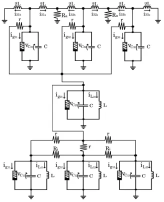
In this study, we investigate synchronization phenomena of van der Pol oscillators of hourglass structure by changing the coupling strengths. We use van der Pol oscillators which are coupled by resistors.
2. System Model
The circuit model of the hourglass structure using van der Pol oscillators is shown in Fig. 1.
C L
ig12
vC12
iL12
C L
ig11
vC11
iL11
C L
ig13
vC13
iL13
C L
ig21
vC21
iL21
ig31
vC31 C
ig32
vC32 C
ig33
vC33 C
Ra Ra
Ri Ri
i31b i31a i32b i32a i33b i33a
r r
2L 2L 2L 2L 2L 2L
r r
r r
Figure 1: Circuit model of Hourglass Structure.
The normalized circuit equations of this circuit equations are given by the following equations.
(1) Bottom oscillators:
˙
x11=εx11(1−x112
)−y11
−αi(x11−x12)−β(x11−x21)
˙ y11=x11
˙
x12=εx12(1−x122
)−y12
+αi(x11−2x12+x13)−β(x12−x21)
˙ y12=x12
˙
x13=εx13(1−x132
)−y13
−αi(x13−x12)−β(x13−x21)
˙ y13=x13
(1)
(2) Middle oscillators:
˙
x21=εx21(1−x212
)−y21
+β(x11+x12+x13−6x21+x31+x32+x33)
˙ y21=x21
(2)
(3) Top oscillators:
˙
x31=εx31(1−x312
)−(y31a+y31b)−β(x31−x21)
˙
y31a= 0.5x31−αa(y31a+y32b)
˙
y31b= 0.5x31
˙
x32=εx32(1−x322
)−(y32a+y32b)−β(x32−x21)
˙
y32a= 0.5x32−αa(y32a+y33b)
˙
y32b= 0.5x32−αa(y31a+y32b)
˙
x33=εx33(1−x332
)−(y33a+y33b)−β(x33−x21)
˙
y33a= 0.5x33
˙
y33b= 0.5x33−αa(y32a+y33b)
(3)
The parameter β corresponds the coupling strength be- tween the circuits.
3. Simulation results
In this study, we change the coupling strengths of the resistors connected to the middle van der Pol oscillator.
Figure 2 shows the computer simulation results. The circuit parameters are chosen asε= 0.10,αi=αa= 0.5 , and β= 0.02.
In this result, we have confirmed that all circuits are syn- chronized when the coupling strengths areβ= 0.02. On the other hand, we have confirmed anti-phase synchronization only at x32 while nearly all circuits are synchronized with in-phase.
11
11 11
12 13
11 11
21
11 11 11
32 33 31
x
x x
x x
x x
x x
x x
x x
x
Figure 2: Computer simulation results (phase shift)
4. Conclusion
In this study, we investigated synchronization phenom- ena of the hourglass structure using van der Pol oscillators.
As our future works, we will confirm the synchronization phenomena by changing the coupling strengths of the resis- tors connecting the top and bottom van der Pol oscillators and increasing the number of van der Pol oscillators in the middle.
15