鹿児島大学リポジトリ

Numerical Calculation of Tide in Kagoshima Bay

: Part 1. Two Dimensional Explicit Method

著者

KIKUKAWA Hiroyuki, KURIYAMA Shoji

journal or

publication title

鹿児島大学水産学部紀要=Memoirs of Faculty of

Fisheries Kagoshima University

volume

29

page range

169-177

別言語のタイトル

鹿児島湾潮汐の2次元数値模型

Vol.29 pp. 169-177 (1980)

Numerical Calculation of Tide in Kagoshima Bay

Hiroyuki Kikukawa* and Shoji Kuriyama*

Abstract

The tide in Kagoshima bay is calculated by an explicit two dimensional numerical method. For the time differentiation, the two-step Lax-Wendroff difference method is adopted and for the space, the two dimensional finite element method is used. The estimated tidal residual flow shows the existence of three large vortices in Kagoshima bay, i.e., clockwise vortices at south and north of Nishi-Sakurajima channel and an anti-clockwise vortex at the center of the bay. These vortices qualitatively agree with the experimental ones.

1. Introduction

Water exchange in a semi-closed bay is essential for the environment of fish cultures and especially for comfortable human lives around the bay. In addition to experi mental investigation, we believe, the numerical model calculation is respectable to make clear the primary factors of the water exchange in the bay. Kawaharada

et al.1) investigated the tidal current in Kagoshima bay by using one dimensional

implicit model and showed that the tidal current induces only rather small movement of water mass. Although the one dimensional model is much advantageous eco

nomically, geographical features can not be accounted in this scheme. In this paper, we improve their analysis to the two dimensional model by applying an explicit

numerical method. Recently, explicit numerical method is shown2) to be more appropriate than the implicit one in order to solve the hyperbolic type differential equation. According to Kawahara et al.3>, we adopt the two-step Lax-Wendroff

difference method4) for the time differentiation and divide the surface of the bay by

the two dimensional simplex elements.

The water exchange is caused by the tidal residual flow, the density current and the wind-driven current. The last two effects can be rightly estimated only by the three dimensional formulation5^. The three dimensional calculation have to be finally performed. It requires, however, large capacity of a computer and long computational time. Even the two dimensional estimation could give the rough features of the water exchange in the bay, especially if the water in the bay is stratified

and the wind blows gently.

In section 2, we give the formulation. Results are given in section 3. Section 4

is devoted to discussions.

170 Mem. Fac. Fish., Kagoshima Univ. Vol. 29 (1980)

2. Formulation

For complete fluid, Euler's equations of motion and equation of continuity are

written as: du _ i _ , d u . d u . d 7 ) r n dt dx dy dx dv . dv , dv . dri . r n

9y , 9(giQ , 9(ffo) _Q

dt ^

dx

^

dy

where wand y are vertically averaged water velocities of x and j; directions respectively,

rj is the water elevation, H=h-\-iq with A denoting the depth, g is the gravitational

constant and/is the Coriolis parameter. In order to solve Eqs. (2.1)—(2.3) numeri cally in the bay, we first divide the surface of the bay by the two dimensional simplex element (see Fig. 1). Concentrating on one of the elements and following the usual formulations of the method of weighted residuals6) we consider in that element, the

variational functionals:

Fig. 1. Division of Kagoshima bay by the two dimensional simplex elements.

wy)dA-^=L'*(

(2.4)

(2.5)

where dA denotes the two dimensional integral and u*, v* and 37* are weighting functions.

Assuming linear dependences on coordinates for u, v, -q and h in a simplex element,

it follows:

? = 9tfZfl.(a= l-3),.

, (2.7)

where q represents u, v, 37 and h and summation convention is used. In Eq. (2.7) qa

is the value of q at the a-th vertex of the triangle and La (a=1-3) are the barycentric

coordinates:

£*= 2j(a>a +bax +cay)9

(2.8)

where A is the area of the simplex element and

ca= x7-xfi. (a9 /?, r cyclic)

(2.9)

According to the Galerkin's method, weighting function q* representing u*, v* and

37* is also written as:

•-q* = q*La(a = l;~S), .:

(2.10)

where q% is the arbitrary variation at the a-th vertex of the triangle element. Sub stituting Eqs. (2.7)-(2.10) into Eqs. (2.4)-(2.6) we obtain:

dxeu = it* \ (LaL/3u/3 + LaL/3L7iXU0U7 + LaL/3L7tyv/3u7

+ gLaLfitX7)p -fLaLpVp) dA9

(2.11)

dxev =v* J (LaLpVp +LaL^L7fXu^v7 +LaL^L7tyv^v7

+ gLaLfityv0+fLaLfiufi)dA9

(2.12)

+ LaLfit9L7Hj,v7 + LaL^L7t yH^v7) dA, (2.13)

where

Ha=ha + iqa.,

We require the functionals 8Xeu, 8X% and 5Z« vanish for arbitrary u%, v* and rj%.

The time developments of u[, v and 37 are given by using thie two-step Lax-Wendroff

172 Mem. Fac. Fish., Kagoshima Univ. Vol. 29 (1980)

7»+|_/7» . At A

T= ?"+-^L?nJ

(2.14)

i

qn+1 = q» + Jtqn+T. (2.15)

Our final equations for one element are given by:

+ gm^%-fMa0v%),

(2.16)

Maev%+1 =Maev%- ^-(K'affyu%v!}+Kiffyv»^

+ gWaerfl+fMa/3u«fl)

(2.17)

Ma/3y%+ 2=Matf%- 4f- {K*aff7(H0u7 +u%H«)

+K>a0y(Hf}nv»+v%H!})},

(2.18)

+ gNUVn^-fMaBv^k),

(2.19)

Maf>vpi = Mal3v% - AKKle,u%+1zvf t +Ki$yvf\v»+ J

+ gNya/3y%+Jl+fMa0u"/h

(2.20)

+KZf)y(H»0Hv7+ t +t,J+i fl*4 )>,

(2.21)

Mafi=^ LaLfidA9

Ka&f— \ LaLpL7XdA9

Kyap7= \ LaL/3L7ydA9

J A J A

N'a$=^ALaL0tXdA, Nie=^LaL0iydA.

(2.22)

The integrals in Eq. (2.22) are easily performed by using the formula7':

ALfLlLidA= ^f?+2),2A.

(2.23)

S

As the matrix M is not a diagonal one, q%+l12 and q%+1 can not be solved explicitly.

We then adopt the lamped mass matrix technique85, that is, instead of the original

mass matrix M in the left-hand sides of Eqs. (2.16)—(2.21) we use the diagonal mass matrix in which all of the off-diagonal elements are summed to the diagonal ones. Owing to this technique our scheme becomes completely explicit.

By summing Eqs. (2.16)—(2.21) over all elements, the velocities and elevations of

all nodal points at time / can be explicitly calculated if those at time t—At are known.

3. Results

Our division of Kagoshima bay by the two dimensional simplex elements is given in Fig. 1. The numbers of element and nodal point are 417 and 255, respectively. We have carefully divided the bay to use only acute type triangles. In the explicit

numerical method, the time step is limited95 by the inequality:

At£ Ax

fgH

Nishi-Sakurajima channel gives the upper limit of At to be about 50 seconds. For safety, we have chosen 30 seconds for the time step. As our purpose is the model calculation, we give the sine curve with amplitude 1.0 meter and period 12.5 hours for the elevation at the entrance of Kagoshima bay. We adopt the slip boundary condition, i.e., the velocity perpendicular to the shoreline vanishes. Initial condition is that the vertically averaged velocities at all nodal points are vanished and the surface of the bay is flat. The real depths at all nodal points are read out from the chart and utilized.

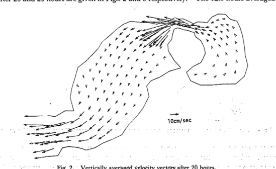
Calculation was performed over 30 hours. . The vertically averaged velocity vectors

after 20 and 26 hours are given in Figs. 2 and 3 respectively. The 12.5 hours averaged

lOon/sec

174 Mem. Fac. Fish., Kagoshima Univ. Vol. 29 (1980)

lOcm/sec

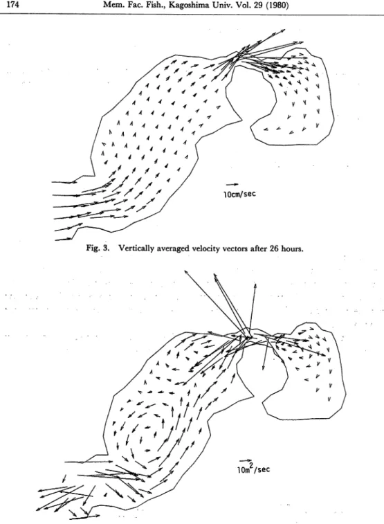
Fig. 3. Vertically averaged velocity vectors after 26 hours.

10m /sec

Fig. 4. Sum of the vertically averaged velocity vectors times their depths //oyer the last 12.5 hours.

mass transport (vertically averaged velocity vectors times their depth.// (=h+yj)) is

shown in Fig. 4. Three large vortices can be seen in the figure, i.e., clockwise vortices

Fig. 5. Elevations at (A), (B) and (C) shown in Fig. 1.

center of the bay. The experiment10) also seems to show such vortices. The ele vations at the entrance (A) (close to our input), at the off Kagoshima city (B) and off Fukuyama city (C) are given in Fig. 5. The phase differences of (B) and (C) with respect to (A) can be seen to be about 20 and 90 minutes respectively. The prelimi nary experiment at the coast of Fukuyama city implies that these values are larger

than the experimental ones. We have to perform more careful experiment to see

whether the disagreement is fateful or not. The amplitude of (B) is 4% larger and that of (C) is 7.5% smaller than the amplitude of (A).

4. Discussion

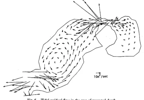
Recently Morihira et al.n) implied that in the ocean with violently varied depth, it is desirable for the two dimensional calculation of tidal current to ignore most

10m /sec

176 Mem. Fac. Fish., Kagoshima Univ. Vol. 29 (1980)

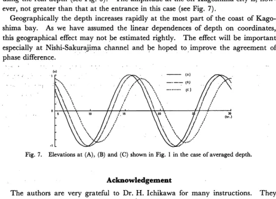
deep place. According to them, we tried to ignore the depth deeper than 80 (60) meters in the southern (northern) place of Nishi-Sakurajima channel. The resulted tidal residual current does not change so much compared with the result of calculation using the real depth (see Fig. 6). The amplitude at the off Kagoshima city is, how ever, not greater than that at the entrance in this case (see Fig. 7).

Geographically the depth increases rapidly at the most part of the coast of Kago shima bay. As we have assumed the linear dependences of depth on coordinates, this geographical effect may not be estimated rightly. The effect will be important especially at Nishi-Sakurajima channel and be hoped to improve the agreement of phase difference.

Fig. 7. Elevations at (A), (B) and (C) shown in Fig. 1 in the case of averaged depth.

Acknowledgement

The authors are very grateful to Dr. H. Ichikawa for many instructions. They

also wish to thank Lecture Y. Matsuno for his kindness to show the chart and for

instructions to reading it. The computation was carried out in FACOM M-200 of Computer Center of Kyushu University.

References

i) M®ffl*L#cfl$, pmm% • Mm *& (1976,1980): rt«»*©»iiii»co^-c(o*3i*fl9W3ti,n, 2) H. Fujn (1972): Finite elementschemes: stability and convergence, Advances in Computational

Method in Structual Mechanics and Design, HAH Press, 201-218.

A, ttMm, »*#* (1976) :2a»^y^^-^xVKn7*R5*ft»C<kS«IiJr«E

SS230Mmn^mm&m-zm, 498-501.

R. D. Richtmyer (1963): A survey of difference methods for non-steady fluid dynamics, N. C. A. R. Tech. Note, 63-2.

•XWttM (1979) :*SR«(Dfi*ICH-rS*«[**, m6®MmX¥M&&mXM, 514-518.

J. Sudermann (1977) : Computation ofbarotropic tides by the finite elementmethod, Int. Conf.

Finite Element Water Resour., 51-67.

L. J. Segerlind (1976): Applied Finite Element Analysis, John Wiley & Sons. O. C. Zienkiewicz (1977): The Finite Element Method, 3-rd Eddition, McGraw-Hill. 3) ill

4)

5)

7) M. A. E. Eisenberg and L. E. Malvern (1973): On finite element integration in natural co

ordinates, Int. Jour. Numer. Meth. in Eng. 7 574-575. 8) See O. C. Zienkiewicz in ref. 5, 535-539.

9) A. F. Blumberg (1977): Numerical modelor esturine circulation, Jour. Hydraul. Div. ASCE 103

295-310.

io) miom%.M±u%*u (1977): mftmomm.

id «¥«&&, mi n, &«*s, mmm*, nmmA (1979): m&^mm*m^tzM®<D=ik7t