An Application of Modular approach to
Separable Nonlinear Programming Problem
岡山理科大学 岩崎 彰典 (Akinori Iwasaki)
四国大学 疋田 光伯 (Mitsunori Hikita)
岡山理科大学 仲川 勇二 (Yuji Nakagawa)
岡山理科大学 成久 洋之 (Hiroyuki Narihisa)
Abstract
A discrete optimization method, which is called modular approach, is proposed for solving a
separable nonlinear programming problem. By dividing seach space ofvariables, the nonlinear
pro-gramming problemis translated into a discrete optimization problemthat isequivalentto nonlinear
knapsack problem. When the nonlinear knapsack problem issolved, we do not need the convexity
anddifferentiabilityoforiginalproblem. Thenonlinear knapsack problemcan besolvedefficiently by
modular approach. It is shown that modular approach can be applied to a nonlinear programming
problem by computationalexperiments.
1. Introduction
A separable nonlinear programming problem with one constraint
func-tion is written as follows:
$<N>$
maximize $f(x)= \sum_{i\in I}f_{i}(x_{i})$, (1) subject to $g(x)= \sum_{i\in I}g_{i}(x_{i})\leq b$, (2) $x_{i}\in s_{i}$ $(i\in I)$, (3)
where $I=\{1,2, \ldots, n\}$, and $S_{i}\subset R$ is a seach space, and $b$ is a maximum
amount of available resource.
We divide the seach space $S_{i}$ into finite set $A_{i}$ for each i–th variable:
$<K>$
maximize $f(x)= \sum_{i\in I}f_{i}(x_{i})$, (4)
subject to $g(x)= \sum_{i\in I}.g_{i}(x_{i})\leq b$, (5)
$x_{i}\in A_{i}$
.
where $I=\{1,2, \ldots, n\},$ $A_{i}=\{a_{i1}, a_{i2}, \ldots, a_{ij}, \ldots, a_{ik_{i}}\}$. The search
space $S_{i}$ is represented by $k_{i}$ points $\{a_{i1}, \ldots a_{ik_{i}}\}$.
The original problem $<N>$ is translated into discrete optimization
problem $<K>that$ is equivalent to thenonlinear knapsack problem. Solv-ing the nonlinear knapsack problem by discrete optimization method, the convexity and differentiability of original problem are not required.
We use modular approach(MA) for solving the nonlinear knapsack
problem $<K>$. MA can solve the large scale nonlinear knapsack problem.
The optimal solution of the problem $<K>is$ a near optimal solution of
the original problem $<N>$. The search space $S_{i}$ of the original problem
can be reduced to the neighborhood of the near optimal solution. The
new problem with reduced search spaces is created and solved by MA. By
repetition of the above procedures, the near optimal solutions conyerge
into the optimal solution of original problem $<N>$.
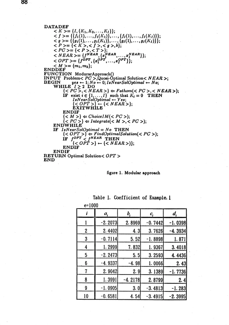
2. Modular approach
Nakagawa[l] proposed a new solution method called modular approach (MA) for solving discrete optimization problem. MA is a bottom-up scheme as well as Dynamic Programming. First, MA considers an opti-mization system corresponding to a given discrete optimization problem.
Next, MA executes the following items 1) 2) recursively until the number
of variables $I$ becomes one.
1) The set $A_{i}$ is reduced by fathoming tests.
2) Integrate two variables into one variable.
As for fathoming tests, we use dominance test, $boundin^{\backslash }g$ test and
feasi-bility test, which are techniques commonly used by Branch-and-Bound.
to cartesian product of the two sets as follows:
$A_{NEW}=A_{j}\cross A_{m}$ (7)
and $j$ and $m$ are removed from the set $I$.
There are four ways to select the sets $j$ and $m$ in the set $I$. Let $k_{i}$ be
the number of elements in the set $A_{i}$.
1) $j$ and $m$ such that $k_{j}$ and $k_{m}$ are the least.
2) $j$ such that $k_{j}$ is the least, and $m$ such that $k_{m}$ is the most. 3) $j$ and $m$ such that $k_{j}$ and $k_{m}$ are the most.
4) $j$ and $m$ in order of $i\in I$.
We choose the item 2) that is the fastest and can solve the largest scale problem. [3]
MA written by pseudo code is shown in figure 1.
The input of ModularApproach$()$ is a data sequence of Problem
$<PC>$
and Quosi-Optimal Solution$<NEAR$
$>$. Problem$<PC>$
contains adata sequence of current problem $<P>$ and a data sequence of $<T>$ that is required to translate the current problem $<P,$ $>$ into primal
problem. The Quosi-Optimal Solution
$<NEAR>is$
given by Recursive Greedy method[2]. Function Fathom$()$ reduces the set $A_{i}$ by fathomingtests, and renews the current problem
$<P>$
. Function ChoiceIM$()$ selects two sets $A_{j}$ and $A_{m}$. Function Integrate$()$ integrates the two sets$A_{j}$ and $A_{m}$ into one set $A_{NEW}^{\backslash }$. After repeating the fathoming tests and
integration, function FindOptimalSolution$()$ gives the optimal solution
of the one variable problem.
3. Computational experiments
We divide the serch space $S_{i}$ of given problem into finite set $A_{i}$ . We create the nonlinear knapsack problem from the set $A_{i}$. The next two
steps are repeated until required precision is given.
1) MA is applied to the nonlinear knapsack problem, and near optimal solution of given problem is given.
2) The neighborhood of the near optimal solution is divided, and the new nonlinear knapsack problem with reduced seach spaces is created.
3.1 Example 1
We consider a convex and differentiable problem as follows:
maximlze $f(x)= \sum_{i=1}^{10}(a_{i}+b_{i}x_{i})^{2}$, (8)
subject to $g(x)= \sum_{i=1}^{10}(c_{i}+d_{i}x_{i})^{2}\leq e$, (9)
$x_{i}\in R$. (10)
Coeficients $a_{i},$ $b_{i},$ $c_{i},$ $d_{i}$ and $e$ are shown in Table 1.
This problemis solved bynumerical computation and MA. Each results
are shown in Table 2. Generally the results of MA are agreement with
the results of numerical computation.
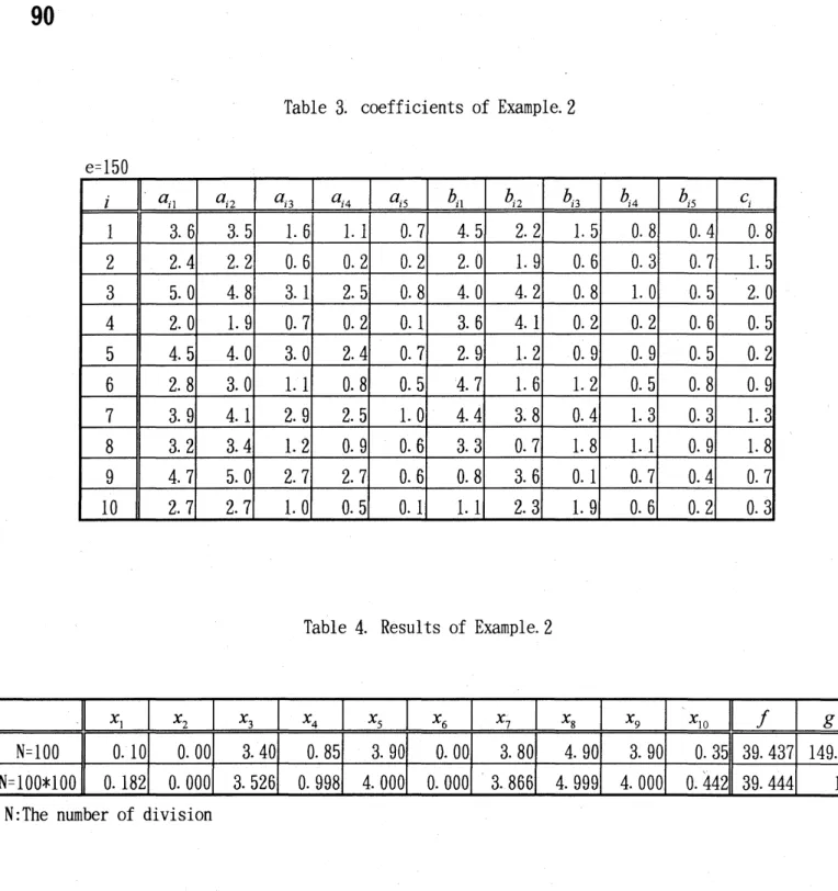
3.2 Example 2
We consider the nonconvex and undifferentiable problem as follows: maximize $f(x)= \sum_{i=1}^{10}f_{i}(x_{i})$, (11)
subject to $g(x)= \sum_{i=1}^{10}g_{i}(x_{i})$, (12)
$g_{i}(x_{i})=(x_{i}+c_{i})^{2}\leq e$. (14)
Coefficients $a_{i1},$
$\ldots,$$a_{i5},$$b_{i1},$ $\ldots,$$b_{i5},$ $c_{i}$ and $e$ are shown in Table 3.
This problem is solved by MA and the results are shown in Table
4. First, the seach space is divided into 100 elements, and the near
optimal solution is given by MA. Next, the neighborhood of the near
optimal solution is divided into 100 elements, and the second near optimal solution is also given by MA. The second near optimal solution exhausts
the resource of constraint. 4. Concluding remarks
Solving two examples, it is shown that MA can solve nonconvex and undifferentiable nonlinear programming problem.
References
[1] Nakagawa Y.: A New Method for Discrete optimization Problems”,
Trans. IEICE, Vol.J73-A No.3 pp $55^{}0- 556$ (1990)
[2] Nakagawa Y.,Ohtagaki.$H:$ A modification of greedy procedure for
solving nonlinear knapsack class of reliability optimization
prob-lems”,
Trans. IEICE, Vol.J74-A No.3 pp.535-541 (1991)
[3] Nakagawa Y.,Hikita T.,Iwasaki A.: A Fast Exact Method for the Multiple Choice Knapsack Problem”,
$DAT_{<K}ADE_{>}F_{=\{I,\{K_{1},K_{2},\ldots,K_{J}\}\};}$ $<f>=ttf_{1}(1),\ldots,f_{1}(K_{1})\},\ldots,\{f;(1),\ldots,h(K_{J})\}\}$; $<g>=\{\{g_{1}(1),\ldots,g_{1}(K_{1})\},\ldots,\{g_{l}(1),\ldots,gr(K_{l})\}\}$; $<P>=\{<If>,<f>,<g>,b\}$; $<PC>=\{<P>,<T>\}$; $<OPT>=tf^{OPT}t^{x_{1}^{\acute{O}PT^{NB.4R}},..,x_{i}^{OPT’}\}\}}<NEAR>--\{[NB\lambda R\{x_{1\prime}\ldots x^{N.BlR},\}\}$; $END^{<M}DEF^{>=\{m_{1},m_{2}\};}$
$BEGI^{TProb1em<PC>,Qu\circ.si-\int)}INPU_{Nyarrow}FUNCTIONModurarAroac_{d_{earSolOp\lim alarrow No}^{tima1S\circ 1ution<NEAR}}esarrow 1,\cdot No^{pph}0,Is,>j$
WHILE $I>2$ DO
$t<PC\overline{>},$$<NEAR>$} $\Leftarrow Fathom(<PC>, <NEAR >)$;
IF $e_{I^{isti\in}}x_{sN\epsilon ar}1_{ol’\dot{O}p\iota imalarrow Yes;}^{1..,I\}suchthatK_{j}=0}$ TIIEN
$t_{XITWH}^{<OPT>}\}_{LE}^{arrow\{<NEAR>\}}$, $ENDIFt<M>\}\Leftarrow Choic\epsilon IM(<PC>),\cdot$
$t<PC>\}\Leftarrow I$ leg$\cdot at\epsilon(<M>, <PC>)$;
ENDWHILE
IF $IsN\epsilon arSolOptimal_{1}=NoTHENt<OPT>1\Leftarrow Fi\iota dOplir|\iota alSolu\ell io|\iota(<PC>)$
;
$IFf^{OPT}<f^{NB\lambda R}ENDIFt<OPT>1arrow t<NEAR>)\};THEN$
ENDIF
ENDRETURN
Optimal $Solution<OPT>$figure 1. Modular approach
Table 3. coefficients of Example.2
Table 4. Results of Example.2