Note on dynamically stable perturbations of parabolics (Complex Dynamics)

(1)

90 Note

on

dynamically stable

perturbations of

parabolics

Tomoki Kawahira

*

Nagoya University

[email protected]

Abstract

Inthisnote,we sketchsome results onalmost-dynamics-preserving

per-turbationsofrational maps with parabolic cycles.

1 Introduction with rabbits

Well known “

$\mathrm{D}\mathrm{o}\mathrm{u}\mathrm{a}\mathrm{d}\mathrm{y}^{)}\mathrm{s}$ rabbit” has a friend called (“fat rabbit” at the root of

1/3-limbof the Mandelbrot set. Howeverthe term “fat” does not sound good,

so

we

tentatively call him “chubby rabbit”.

$|$

Figure 1: “plump”, “chubby” , and “overweight”.

“Chubby rabbit” has a parabolic fixed point with

3

petals and multiplier

$e^{2\pi \mathrm{z}/}?.$. Actually there is anoverweight rabbit in the main cardioid, which has an

attractingfixedpointwithmultiplierof theform$rc^{2\pi i/3}(0<r<1)$. Onthe other

hand, there is a little bit thinner rabbit than $” \mathrm{c}\mathrm{h}\mathrm{u}\mathrm{b}\mathrm{b}\mathrm{y}^{\grave{\prime}}$’

near

“Douady’s , which

’The author gave a talk on 20 February 2003 at RIMS, Kyoto this note is written for

RIMS Kokyuroku

(2)

$\theta$$1$

has a repelling fixed point with multiplier $Re^{2\pi i/3}$ $(R >1)$. So

we

tentatively

call them “overweight rabbit” and “plump rabbit”. (Idon’t know whether these

terms

are

proper

or

not, though...)

The change from “chubby” to “overweight”

or

“plump” is parameterized by the multiplier of $(\alpha-)\mathrm{f}\mathrm{i}\mathrm{x}\mathrm{e}\mathrm{d}$ point. They look similar when $r$ and$R$

are

very close

to 1 (Figure 1). Actually “overweight” and “plump” converge to “chubby”

as

$r$,$Rarrow 1$ in the HausdorfTtopology. Moreover, the dynamicsonthe Juliasetsare

almost the

same

as

we can

see

byobservingthe combinatorics oflanding external rays. (By theoremsin

52,

we

can

also

see

that the dynamicsinside the Juliasets

are

almost the same.)

In thle general case, changes from “parabolic” to “hyperbolic” ($=$ attracting

orrepelling ), or oppositedirections,

are

noteasy

as

above. Thedifficulty

com es

from well-known parabolic implosion, but herewe omitto deal with it. Our main question is:

For a rational $\tau nap$ with a parabolic cycle,

can we

give a $wa?/$ to

perturb itsparabolic cycle into another kind

_of

cycle without changing

most part

_of

the dynamics$p$

In this note,

we

willgive a quick survey

on

this proble $\mathrm{m}$.

1.1 Preliminary

Here we list

some

definitions and notation.

Classes of rational maps, Let $f$ : $\hat{\mathbb{C}}arrow \mathbb{C}\mathrm{A}$

be a rationalmap of degree $d\geq 2$.

Here we recall

some

famous classes:

.

$f$ isgeometrically

finite

if every critical point in the Julia set$J(f)$ is

PrePe-riodic. If$f$ isgeometrically finite, theFatou set $F(f)$ consists of attracting

or parabolic basins.

.

$f$is called subhyperbolic if$f$ is geometricallyfinite without parabolic cycles.

$\bullet$ _$f$ is called subhyperbolic if$f$ has

no

recurrent criticalpoints

nor

parabolic

cycles in its Julia set.

In

\S 3, we

will deal with

one

more class ofrational maps, called weakly hyper-bolic.

Perturbation. A perturbation of a rational map (resp. polynomial) $f$ is

a

family of rational maps (resp. polynomials) $\{f_{\epsilon} :\epsilon\in[0, c_{0}]\}$ with

some

$\epsilon_{0}>0$

satisfying $f_{0}=f$ ). $\deg f_{\epsilon}=d,\cdot$ and $d_{\hat{\mathbb{C}}}(f_{\epsilon}, f)arrow \mathrm{O}$

as

$\epsilonarrow 0$. For simplicity, we

(3)

82

Notation.

.

For aparabolic or attracting periodic point $\alpha$, $A(\alpha)$ denotes its immediate

basin.

.

$P(f)$ denotes the postcritical set of$f$.

.

$C(f)$ denotes the criticalset of$f$.

2 Polynomial

case:

Theorems

of

P.

$\mathrm{H}\dot{\mathrm{a}}\mathrm{i}\mathrm{s}\mathrm{s}\mathrm{i}\mathrm{n}\mathrm{s}\mathrm{k}\mathrm{y}$

In the case ofpolynomial, there

are some

results by Peter Haissinsky. Here we

sketch his sequential workrelatedtoour question. In thissection we

assume

that $f$ is a polynomial of degree $d\geq 2$

.

2,1

_Parabolic

_to

_repelling

The first theorem is on a perturbation of direction $” \mathrm{p}$ arabolic$arrow$ repelling”.

Theorem 2.1 (Haissinsky, [5])

_If

$f$ isgeometrically

finite

with connected Julia

set, then there exists apolynomial perturbation $f_{\epsilon}arrow f$ accompanied by

conjuga-cies between the actions

of

the Julia sets. Moreover, $f_{\epsilon}$ are all subhype rbolic.

This theorem is extended later in

\S 3.

Sketch of the proof. The last sentence implies that every parabolic cycle in $J(f)$ is perturbed into

a

repelling cycle. We explicitly construct a rational

perturbation $F_{\epsilon}=f+\epsilon R$, where $R$ is a rational function which takes value

zero

at all parabolic cycles and at finite critical orbits on $J(f)$. (Here

we

allow

$\deg F_{\epsilon}\geq\deg f.)$ Then $F_{\epsilon}$ has cycles exactly the

same

places

as

the original

parabolic cycles, buttheir multipliers are changed slightly by $R$. Here

we

take a

proper$R$to make them repelling. Moreover, topreservethe local degree of critical

orbits

on

the Julia sets,

we

take $R$ to have enough tangency at those points. If

$\epsilon$ $\ll 1$, we can take a nice topological-disk neighborhood $U$ of $J(f)$ such that $\{U, F_{\epsilon}^{-1}(U), F_{\epsilon}\}$ is an analytic family ofpotynomia1-4ii$\mathrm{e}$map. By straightening,

we

obtain a subhyperbolic perturbation $f_{\epsilon}arrow f$. Now it is known that the

connected Julia sets of geometrically finite polynomials

are

locally connected.

Thus every externalrayland on thhe Juliasets. To check thedynamical stability

on

the Julia sets,

we

check the stability of the ray equivalence, which is defined

(4)

83

Goldberg-Milnor conjecture. Theorem 2.1 gives

an

affirmative answer to the following Goldberg-M ilnor conjecture in the

case

ofgeometrically finite poly-nolnials: For a polynomial $f$ which has a parabolic cycle, there exists a small perturbation

_of

$f$ such that

.

the immediate basin

_of

the parabolic cycle is converted to basins

of

some

attracting cycles; and

.

the perturbed polynomial on its Julia set $\iota s$ topologically conjugate to the

original polynomial$f$ on$J(f)$.

Conversely,is it possible to create parabolics from hyperbolics(attractingor

repelling)? The following results give us

some

partial

answers.

2.2 Repelling to parabolic

Next we consider the opposite direction: “repelling $arrow$ parabolic”. The second

theorem is:

Theorem 2.2 $(\mathrm{H}\dot{\mathrm{a}}\mathrm{i}\mathrm{s}\mathrm{s}\mathrm{i}\mathrm{n}\mathrm{s}\mathrm{k}\mathrm{y}, [4])$ Suppose $f$ has an attracting

fixed

point a and

a repelling

_fixed

point$\beta$ on $\partial A(\alpha)$. Vie also add the following condition:

(B) $\beta$ is accessible

from

$A(\alpha)$ and$\beta\not\in P(f)$

Then there exists a polynomial $g$

of

degree $d$ and a homeomorphism $h$ :

$\mathbb{C}$ $arrow \mathbb{C}$

such that

.

$h\circ \mathrm{f}(\mathrm{z})=g\circ h(z)$

for

any $z\in\hat{\mathbb{C}}-A(\alpha)$;

.

$h(\beta)$ is

a

parabolic

fixed

point and $h(A(\alpha))=A(h(\beta))$; and

@ $h|_{J(f)}$ gives a topological conjugacy between the actions on the Julia sets.

We can

remove

condition (B) when $f$ is geometrically finite. Moreover, we

can modify the statem ent by replacing the term “fixed point” with “$\mathrm{c}\mathrm{y}\mathrm{c}1\mathrm{e}^{)}’$.

This theoremsaysthat

we can

convert anattracting basin intothe parabolic basin in

our

particular situation. The conjugacy breaks only on the immediate

basin $A(\alpha)$, where

we

operate tricky surgery by

means

$\mathrm{n}\mathrm{s}$of

$\mu$

-conformal

map. $\mu-$

conforrnal map is not a quasiconformal map, though it is exponentially close to

quasiconformal insome

sense.

Let $\mu$ :

$\mathbb{C}arrow \mathrm{D}$be a measurable function which satisfies

Area{z

$\in \mathbb{C}$ : $|\mu(z)|>1-\in$

}

$\leq Ce^{-\eta/\epsilon}$

for

some

$C\geq 0$ and$\eta>0$. Such a$\mu$iscalledto be in the David class offunctions

on C. Note that $||\mu||_{\infty}$ can be 1 but it is quite close to the situation $||\mu||_{\infty}<1$

(that is,

(5)

84

for a1J $\epsilon<<1$), which will give us a

quasiconformal

map by solving the Beltram

$\mathrm{i}$

equation $\partial_{\overline{z}}\phi=\mu(z)\partial_{z}\phi$

.

Now the maintool is:

Theorem

2.3

(David, [3]) For $\mu$ in the David class, the Beitrami equation

$\partial_{\overline{z}}\phi=\mu(z)\partial_{z}\phi$ has a unique solution fixing

01

and $\infty$.

We call this solution a $\mu$-conformal map. In the proof, we will partially replace

the M\"obius-hyperbolic-like dynamics

near a

and $\beta$by M\"obius-parabolic-like one

and will obtain

a

new topological dynamics $F$ : $\mathbb{C}arrow$ C. Then $\Gamma^{t}$ admits an

invariant $\mu$ which is in the Davidclass, andby solving the Beitrami equation we

will get the desired polynomial $g$.

Sketch of the proof. For simplicity

we

assume

that $A(\alpha)$ contains

a

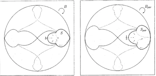
single

critical point only. Then the dynamics in $\Lambda(\alpha)$ is quasiconformally conjugate to

that of a Blaschke product $B$ : $\mathrm{D}$ $arrow \mathit{1}\mathrm{D}$ of the form $B(z)=(z^{2}+b)/(1+bz^{2})$

with $0<b<1/3$

.

Let $\Psi$ : $\mathrm{A}(\mathrm{a})arrow \mathrm{D}$be the conjugacy. By comparing with the

dynamics of $B_{par}(z)=(z^{2}+1/3)/(1+z^{2}/3)$, we will find invariant “sectors” $S$

and $S_{par}$ which have similar dynamical behavior

on

their boundaries (Figure 2).

Indeed, there is a piecewise quasiconformal homeomorphism $\psi$ : $\mathrm{D}$ $arrow \mathrm{D}$ which

satisfies$\psi(S)=S_{par}$ and $\psi$_{$\circ B=B_{par}\circ\psi$} on $\mathrm{D}$$-S$

.

Figure

2:

Dynamics of$B$ and $B_{\mu \mathrm{z}r}$

on

D.

$\Gamma 1^{\urcorner}\mathrm{h}\mathrm{e}$ thickest

curves

show the boundary

of invariant “sectors” $S$ and $S_{par}$. Thinner

curves

show their first and second

preimages.

Now

we

define the topological endomorphism $F\cdot$ $\mathbb{C}arrow \mathbb{C}$ by $F:=P$ on $\mathbb{C}-\mathrm{A}(\mathrm{a})$; and by $F$ $;=(\psi\circ\Psi)^{-1}\circ B_{par}\mathrm{o}(\psi\circ\Psi)$

on

$\mathrm{A}(\mathrm{a})$. (Here

we

replace the

hyperbolic dynamics by parabolic one.) Let$\sigma_{0}$be thestandard complexstructure

of$\mathbb{C}$, and let

(6)

\S 5

a by $\sigma:=(\Gamma’)^{*}n(\sigma_{1})$

on

$P^{-n}(A(\alpha))$; and by $\sigma:=\sigma_{0}$ elsewhere. Then we have

$\Gamma^{*}\prec\sigma---\sigma$.

We have to

use

the property $\beta\not\in P(f)$ in (B). Actually,

even

if

some

critical

orbits land

on

$\beta$ but the other critical points do not accumulate

on

$\beta$,

we can

show tlat the Beltram $\mathrm{i}$ differential

$\mu_{\sigma}$ induced by a belongs to the David class

(bytakingsuitable$\psi$ above). ByTheorem2.3, thereexists a$\mu_{\sigma}$-conformal$\phi$with

$\phi^{*}\sigma_{0}=\sigma \mathrm{a}.\mathrm{e}.$, and the polynomial$g$ $:=\phi\circ\Gamma^{r}\circ\phi^{-1}$ has the desired properties. $\blacksquare$

2.3 Attracting

to parabolic

Next direction is “attracting $arrow$ parabolic” Before stating the thirdtheorem, let

us

start with an easyexample.

Pinching to be “Chubby”, We

assume

from

now on

that $p$ and $q$

axe

rela-tively prime positive integers. (That is, $(p,$$q)=1$ where

we

allow$p=q=1.$)

Set$\omega$ $:=e^{2\pi i\rho/q}$, andconsider a family ofquadratic polynomial

$\{f_{\epsilon}(z)=(1-\epsilon)\omega z+z^{2} : 0\leq\epsilon<1\}$.

For fixed $0<\epsilon_{0}<1$, the dynamics of $f=f_{\epsilon_{0}}$

near

the origin is conform ally

conjugate to $T$ : $w\mapsto(1-\epsilon_{0})\omega w$. Let 4 denote this local conjugacy. We extend it analytically to $\Phi$ : $A(0)arrow \mathbb{C}$by using the relation$w=\Phi(z)=T^{-n}\circ\Phi$$\mathrm{o}f^{n}(z)$.

Now there

are

$q$ symmetrically arrayed raysjoining 0 and oo whose union is

T-in variant

on

$vJ$-plane. By pulling them back by (I)

$)$

we

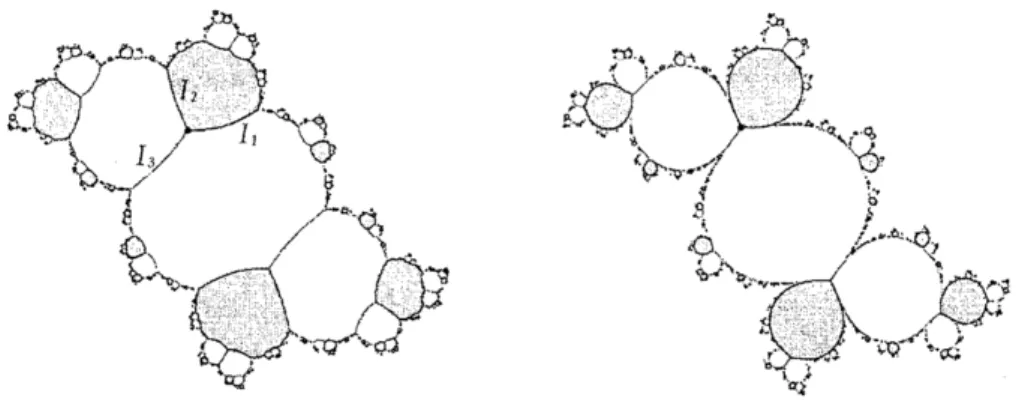
can find $q$ arcs $I_{1}$,

$\ldots\backslash$,$I_{q}$

joining 0 and a repelling cycle $\gamma_{1}$,$\ldots$ ,$\gamma_{q}$, which are permuted by $f$ (That is,

Julia– $J_{j}$ iff$j\equiv \mathrm{i}\dashv- p$modulo $q$) and disjoint from $I^{J}(f)$ (Figure 3).

Figure 3: Left, the Julia set for

an

$f_{\epsilon}$ with $p/q=1/3$

.

Right, the Julia set for $f_{0}$. Shadows distinguish the regions which

never

intersect by the iteration of

$f_{\epsilon}^{3}$

(7)

S6

Set $I:=\overline{\bigcup_{j}I_{j}}$. Bycomparing with the parabolic dynamics of$g=f_{0}$,

one

can

easilyseethat Iof$f$plays the role ofthe parabolic fixed point of$g$, topologically.

Apriori, we can getthe dynam ics of$g$bypinching the grand orbit of$I$. Whatthe

third theorem states is that we canfinda family ofquasiconformaldeformations

$\{f_{\epsilon}\}$ of$f$ which realizes the pinching as above, and

we

can get $g$ as its limit.

Theorem 2.4 $(\mathrm{H}\dot{\mathrm{a}}\mathrm{i}\mathrm{s}\mathrm{s}\mathrm{l}\mathrm{n}\mathrm{s}\mathrm{k}\mathrm{y}, [6])$ Suppose

f

issemihyperbolic withconnected

Ju-lia set and an attractzng

_fixed

point $\alpha$. Then the following holds:

1. For any $p$ and $q$

as

above, there exist $q$ arcs $I_{1},$. .

)$I_{q}$ joining

a

and $a$

repelling cycle

_of

period$q$ permuted by$f$ as the example above.

2. There exists apolynomial$g$ with

a

parabolic

fixed

point$\beta$

of

multiplier$e^{2\pi ip/q}$

which

_satisfies

the following;

.

There exist quasiconformal

_deformations

$\{f_{\epsilon} :0<\epsilon\leq 1\}$

of

$f(=f_{1})$

such that$f_{\epsilon}arrow g$ is aperturbation.

.

Let $H_{\epsilon}$ denote the quasiconformal conjugacy

from

$f$ to $f_{\epsilon}$. Then $H_{\epsilon}$

converges uniformly as$\epsilon$ $arrow 0$ to the limit$h$ which semiconjugates $f$ to

$g$

.

For$y\in\hat{\mathbb{C}}_{f}$ card_{$(h^{-1}(y))\geq 2$} iffy eventually lands on$\beta$. Inparticular,

such an $h^{-1}(y)$ is either $I=\overline{\cup I_{J}}$

or

a connected component

of

its

preimages.

We willsee

some

\S 3.

Idea of the proof. Let us start with a model of pinching and a caricature of quasiconformal deformation. By quasiconformal deformation, we may assume

that the multiplier of$\alpha$ is $\omega/2$. By taking

a

linearizingcoordinate $z\mapsto w$ plus a

covering$w\mapsto(=w^{q}$, the action of $f$ on $\mathrm{A}(\mathrm{a})$ is semiconjugated to $\zeta\mapsto\lambda\zeta$ on $\mathbb{C}$, where A $=(\omega/2)^{q}>0$.

Now we put

an

almost complex structure ($=\mathrm{a}$ field of infinitesimal ellipses)

on

$\mathbb{C}$

as

in Figure 4 By taking the angle $\epsilon$ closer to 0 and making the constant $C_{\epsilon}\nearrow 1$,

we

will have a family of almost complex structures $\sigma_{\epsilon}$ and associating

Beltrami differentials $\mu_{\epsilon}$ which

are

invariant under the action of ( $\vdash*\lambda\zeta$. By

solving the Beltrami equation $\partial_{\overline{\zeta}}\phi=\mu_{\epsilon}(\zeta)\partial_{\zeta}\phi$ for each $\epsilon$, the solution $\phi_{\epsilon}$ fixing

1, $\lambda$, and oo gives a deformation of the quotient torus $\mathbb{C}^{*}/\lambda^{\mathrm{Z}}$ to another torus

with lower modulus. Then quasiconformal map $\phi_{\epsilon}$ converges compact uniformly

to$\phi_{0}$ : $\mathbb{C}^{*}-\mathbb{R}_{-}arrow \mathbb{C}$as$\epsilonarrow 0$, and conjugate theactionof$\langle$ $arrow\lambda\zeta$to$\zeta\mapsto\zeta+1-\lambda$.

Wecanpull-back$\sigma_{\epsilon}$to$A(\alpha)$ by$(z\mapsto w\mapsto\zeta)^{*}$ anddenoteitby

$\sigma_{\epsilon}’$. By putting

$(f^{n})^{*}\sigma_{\epsilon}’$

on

_{$f^{-n}(A(\alpha))$}, and the standard complex structure elsewhere, we have

an

/-invariant almost complex structure and

we

will get afamily of polynomials

$f_{\epsilon}$in the

same

way asthe previous theorem. This mayrealize the pinching $‘(\mathrm{h}\cdot \mathrm{o}\mathrm{m}$

(8)

87

$|_{\mathit{1}’\subseteq}|\nearrow$ $\backslash \backslash _{\backslash \backslash }\backslash$

$\backslash _{\backslash }\backslash$

$|/x_{F}|=c_{\epsilon}^{\backslash _{\backslash }}\backslash \mathrm{E}^{\mathrm{o}}\backslash \acute{\mathrm{C}}\circ\backslash \backslash \dot{\mathrm{o}}_{\mathrm{O}}\backslash \epsilon[_{\Leftrightarrow}\Leftrightarrow\Leftrightarrow\Leftrightarrow\backslash \equiv\backslash \subset=\Leftrightarrow\Leftrightarrow\backslash \backslash \Leftrightarrow\Leftrightarrow \mathrm{a}\Leftrightarrow\fallingdotseq\vee$

$|/4\epsilon|=0$

$\circ 0_{\mathrm{o}\circ \mathrm{s}_{\mathrm{o}\mathrm{o}_{\mathrm{o}_{\mathrm{O}}}^{\mathrm{O}}}^{\mathrm{o}\mathrm{c}}}[mathring]_{\circ}[mathring]_{\mathrm{o}\mathrm{o}^{0\mathrm{O}}}_{\mathrm{o}}^{\mathrm{o}\mathrm{o}^{\circ}}\mathrm{o}\mathrm{o}\circ 6\mathrm{o}_{\mathrm{o}^{\mathrm{o}\mathrm{o}},\circ \mathrm{o}\mathrm{o}\circ\circ}\mathrm{o}\mathrm{c}\mathrm{o}\mathrm{o}$

$\prime\prime/’/$

$|\mu_{\epsilon}|=C_{\acute{\epsilon}}/’/$

$’/^{\prime’}$ $|/x_{\epsilon}|\nearrow$

0 $\lambda$ 1

$|\mu_{\epsilon}|=0$

Figure 4: A caricature of the pinching. On the right half plane $\mu_{\epsilon}(z)=0$. For

$\frac{\pi}{2}<|\arg z|<\pi-\epsilon$, $|\mu_{\epsilon}(z)|$ increases with dilatation $\frac{1+|\mu_{\epsilon}|}{1-|\mu_{\epsilon}|}=1$$+ \tan^{2}(|\arg z|-\frac{\pi}{2})$.

Finally $|\mu_{\epsilon}(z)|$becomesaconstant$0<C_{\epsilon}<1$elsewhere, with$\frac{1+C}{1-C_{\epsilon}}=1+\tan^{2}(.\frac{\pi}{arrow)}-$ $\epsilon)$. Moreover, we take $\arg\mu_{\epsilon}=0$ and $\mu_{\epsilon}$ is constant along any radial lines from

the origin. Hence $\mu_{\epsilon}$ is invariant under

$\langle$$\mapsto\lambda\zeta$.

that the limit of$f_{\epsilon}$as$\epsilonarrow 0$existsandis$g$as wedesired. To check them,wemake

someeffort to show that the integrating map $\phi_{\epsilon}’$ of$\sigma_{\epsilon}’$ is equicontinuous and any

subsequential limits coincide. Inthis technicalpart we

use

the semihyperbolicity of$f$. (We also

use

the weak hyperbolicity of$f$. See

\S 3.)

2.4 Explicit

construction

of pinching: Tessellation

Here we present

an

explicit way of constructing pinching semiconjugacy. The idea is tessellation of filled Julia sets [11]. For simplicitywe explainan example

$\mathrm{j}$ust by figures.

Let

us

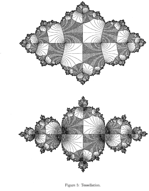
considera family of quadratic polynomials,

$\mathcal{F}=\{f_{\mathrm{c}}(z)=z^{2}+c : -3/4<c<0\}$.

Figure 5 is the pictures of tessellation fortwoquadratics, oneis taken from$F$and

the other is $f_{-3/4}$. The construction oftiles are obviously based on linearizing

coordinates.

Each tile has an “address”,, consists of angle $\theta\in \mathbb{Q}/\mathbb{Z}$, level $n\in \mathbb{Z}$, and

signature $+$ or _-. Addresses are organized so that the tile ofaddress $(\theta,n, +)$ is

mapped to the tileof$(2\theta, n+1, +)$ for example. It matchesto the combinatorics

of external rays, and we

can

preciselydescribe the dynamics inside the Julia set.

Now it is not difficult to

construct

a pinching by pasting tile-to-tile homeo-morphisms which preserve addresses. Then

some

of

arcs

(as $\{I_{j}\}$ inthe previous

example $f_{\epsilon}(z)=(1-\epsilon)\omega z+z^{2})$

are

naturally pinched by continuous extentions of the tile-to-tilehomeomorphisms

(9)

88

(10)

$\theta 9$ 7/3 7/24 5/24 7/6 5/72 $f/7\mathit{2}$ 7,24 $\mathfrak{X}4$ $t7/2\mathit{4}$ 79/24 $f$$7/24t9/24$ 7/12 77/72 2/3 $\gamma$$\gamma/\mathit{2}\mathit{4}$ 79/24 5/6

Figure 6: “Checkerboard” and ((

$\mathrm{Z}\mathrm{e}\mathrm{b}\mathrm{r}\mathrm{a}"$, showing the structure of the addresses

of tiles. “Checkerboard”’, with

some

external rays drawn in, shows the relation

betweentheexternalangles and the angles of tiles. The invariantregions colored

in white and graycorrespond to tiles of signature $+$ and – respectively. $‘\iota \mathrm{Z}\mathrm{e}\mathrm{b}\mathrm{r}\mathrm{a}^{7}$’

shows the levels of tiles. Levels get higher

near

the preimages of the attracting

(11)

100

3 Rational

case:

Geometrically

finite

maps, etc.

Here we deal with the

case

ofrational maps. Some results are natural general-ization of theorems in

52.

3.1

G. Cui’s plumping

deformation.

G. Cui made intriguing applications ofwell-known Thurston rigidity to geom

et-ricaJly finite branched coverings. Here

we

roughly sketch some part of his work relating “parabolic $arrow$ hyperbolic” perturbations. See [1] for his original, or [14]

for a survey of his entire works.

Periodic star-like graphs. Before the main statement, let

us

consider a

ra-tional map $f$ with an attracting cycle$\alpha$of period $l$. For someintegers _$n$, _$m$with

$nm=l$, suppose there axe a repelling cycle $\beta$ of period $n$ and star-like graphs

$I^{1}$,_{$\ldots\}I^{n}$} such that: each $I^{k}$ is centered at arepelling point in$\beta$_). each$I^{k}$ has $\tau n$

feet with their toes at $\alpha,\cdot$ and $f(I^{k})=I^{k+1}$ with superscripts modulo $n$. We call

such an $I^{k}$ a repelling perioiic star-like graph associatedwith $\alpha$.

For example, readers mayimagine the case of “plumprabbit”, withan invari-ant star-like graph connecting the central repellingfixedpoint and the attracting cycle, or the cases of its tuned quadratic polynom ials (i.e. “plump rabbits” in copies of $M$ in $M$). One may call the graph $I=\overline{\cup I_{j}}$in Figure 3 an invariant

attracting stcvr-like graph centered at 0.

Plumping to be “plump”. The theorem here deals with simple plumping,

which replaces parabolic cycles by repelling periodic star-like graphs without

breaking thesymmnletryofpetals, likethe changeof “chubbyrabbit” into‘pplulYlP”.

Now the statement is:

Theorem 3.1 (Cui, [1]) Let g beageometrically

_finite

rationalmapwith parabolic cycles. Then there exists a hyperbolic rational map

_f

satisfying the following:

.

_deformations

$\{f_{\epsilon} : 0<\epsilon\leq 1\}$

of

$f(=f_{1})$ such

that $f_{\epsilon}arrow g$ is aperturbation.

.

Let $H_{\epsilon}$ denote the quasiconfo rmal conjugacy

from

$f$ to $f_{\epsilon}$. Then $fI_{\epsilon}$

con-verges uniformly as $\epsilonarrow 0$ to the limit $h$ which semiconjugaies$f$ to$g$.

.

For$y\in\hat{\mathbb{C}}$, card(h-1

$(y)$) $\geq 2$

iff

$y$ eventually lands

on

a parabolic cycle. In

particular, such an$h^{-1}(y)$ _is either a repellingper iodic star-likegraph or $a$

connected component

_of

itspreimages.

Compare this with Theorem 2.4. (It

was

“overweight” to “chubby”.)

Thistheoremis strongerthanTheorem 2.1 howevertheproof is quitedifferent

(12)

101

branched covering $F$ by replacing all parabolics with proper repelling star-like

graphs. This operation creates

no

Thurston obstruction. Step 2, by a result

on

convergence

of Thurston algorithm in [2],

we can

find

a

subhyperbolic rational

lnap $f$whichis conjugate to$F$. Step

3 we

construct pinching deformations $\{f_{\epsilon}\}$

as

in Theorem 2.4 which has the limit rational map $\hat{g}$ with recreated parabolics.

Step 4, undersuitable normalization of$f$ and $f_{\epsilon}$, we

can

show $g=\hat{g}$by arigidity

result also due to [2].

Actually there is a much stronger theorem which makes Theorem 3.1 just

a corollary. See Theorem $\mathrm{D}+\mathrm{F}’+\mathrm{G}$’ in [14]. Instead of stating it in detail, we

consider anexample.

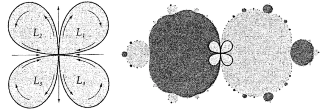
Example (Example 3 of [14]). Set $g(z):=z(1-z^{2})$, with a parabolic at

$z=0$. The attracting (resp. repelling) directions lie

on

$\mathbb{R}$ (resp. $\mathrm{i}\mathbb{R}$). Let $\ell_{1}$ be

an invariant curve in the first quadrant and $L_{1}$ the region enclosed by $\ell_{1}\cup\{0\})$

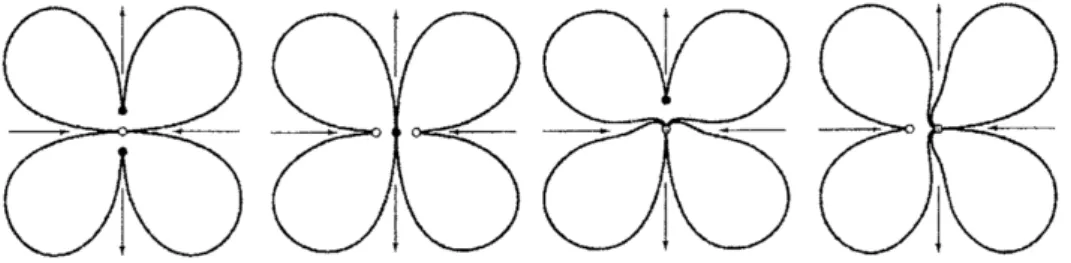
called asepal. For$\mathrm{i}=2,3$, and 4, let$\ell_{i}$ and $L_{i}$ be the symmetricimage of$l_{1}$ and $L_{1}$ in the 2-th quadrant. (See Figure 7.) In particular, $L_{1}$ and $L_{3}$ (resp. $L_{2}$ and $L_{4})$ are called right sepals (resp.

left

sepals).

Figure 7: Sepals and the filled Julia set of $g$.

General plumping is, roughly speaking, replacing

a

pair of right and leftsepals

by

an

invariant

arc

joiningtwo fixed points. To describe possibleways of

PlumP-$\mathrm{i}\mathrm{n}\mathrm{g}$, we consider plumping combinatorics $\tau$

as

following:

$\tau$ is an injective 1nap

defined on $L_{2},$ $L_{4}$, or $L_{2}\mathrm{u}$ $L_{4}$; and $\tau|_{L_{i}}$ $(\mathrm{i}=2, 4)$ is just

a

symmetric reflection

which sends $L_{i}$ to $L_{1}$

or

$I_{3}$, Here is all the possible $\tau$:

(t) $\tau$ : $(L_{2}, L_{4})arrow(L_{3}, L_{3})$

(ii) $\tau$ : $(L_{2}, L_{4})arrow(L_{3}, L_{2})$

(iii) $\tau$ : $L_{2}arrow L_{1}$, $\tau$ : $L_{4}arrow L_{3}$

(13)

102

There are corresponding plunapings of $\tau$ in Figure 8. Two $\tau’ \mathrm{s}$ in (iii) or (iv)

give topologically the

same

plumpings. For example, let

us

pick up a plum Ping

Figure 8: Plumpings of type $(\mathrm{i})-(\mathrm{i}\mathrm{v})$, from left to right. Black, white, and gray

dots show repelling, attracting, and parabolic fixed points respectively

combinatorics $\tau$ : $L_{2}arrow$ U3, that is, $\tau(L_{2})=L_{3}$. Consider

a

Riemann map $\phi$ : $\hat{\mathbb{C}}-\overline{L_{2}\mathrm{U}\tau(L_{2})}arrow\hat{\mathbb{C}}-\overline{\mathrm{D}}$which sends two prime ends at 0 to those of $\pm 1$.

Then there exists a gluing map $T$:C-D $arrow \mathbb{C}$ which identifies the components

of $\partial \mathrm{D}-\{1, -1\}$ such that $T$ respects the holomorphic dynamics

near

$P_{2}$ and

$\tau(P_{2})=\ell_{3}$.

A new plumped map $F$ : $\hat{\mathbb{C}}arrow\hat{\mathbb{C}}$

will be defined basically by $(: \mathrm{o}T)$ $0$

$g\circ(\phi\circ T)^{-1}$. Indeed, it is naturally defined as

an

analytic map except _1ear

$g^{-1}(0)$ $-\{0\}=\{1, -1\}$. T\^a $\mathrm{e}$a small neighborhood$U$ of$\overline{L_{2}\cup\tau(L_{2})}$. Let $U_{1}$ and

$U_{-1}$ be the component of$g^{-1}(U)$ around 1 and -1. Define $F$ on $\phi(U_{\pm \mathit{1}})$ by a

suitable topological map which sends $\partial\phi(U_{\pm 1})$ to $\phi(\partial U)$. Tlen $F$ is a partially analytic $\mathrm{b}1$anched covering.

Cui showed that there exists

a

polynomial $f$ which is conjugate to $F$. More

gcneially,

Theorem 3.2 (Cui) For any plumping combinatorics$\tau$

of

$g$ above, there exists

apolynomial$f$ which is conjugate to apartially analytic map

defined

in asimilar

way as $F$ above. Moreover, there exists

a

quasiconformal

deformation

$f_{\mathrm{c}}(0$ $<$

$\epsilon\leq 1)$

of

$f=f_{1}$ which gives a per rurbation $f_{\epsilon}arrow g_{2}$ and is accompanied by

(semi)conjugacies$f\mathrm{f}_{\epsilon}arrow h$ as in Theorem 3.1.

See [14] for

more

precise statement and the proof, which deals with general geometrically finite rational maps with parabolics.

3.2 Weakly

hyperbolic

maps

In the case of simple plumping, Tan Lei and Hai’ssinsky generalized Step

3

of the proof of Theorem

3.1

to more bigger class ofrational maps

as

following. A

rational map $f$ is weakly hyperbolic if there exist $\delta$ _{$\geq 1$} and $r>0$ with the

following: For any $z\in J(f)$ –

{parabolics},

there exists

a

subsequence $\{n_{l}\iota_{}\}$ of

$\{n\}$ such that

(14)

103

where $B(x_{7}r)$ is a spherical ball of radius $r$ centered at $x_{\backslash }$ and $W_{n}$ is the

com-ponent of $f^{-n}(B(J^{n}(z), r))$ containing $.\sim^{\gamma}$. It is known that semihyperbolic

or

geometricallyfinitemaps

are

weakly hyperbolic.

The statement is:

Theorem 3.3 ($\mathrm{H}\dot{\mathrm{a}}\mathrm{i}\mathrm{s}\mathrm{s}\mathrm{i}\mathrm{n}\mathrm{s}\mathrm{k}\mathrm{y}$and Tan, [8]) Let $f$ be a weakly hyperbolic

ratio-nal map with attracting cycles. Let I be

an

$f$-invanant collection

of

periodic repelling star-like graphs associated with the attracting cycles. Then there exists

a rational map$g$ with parabolic cycles which

satisfies

the following:

.

defo

relations $\{f_{\epsilon} : 0<\epsilon\leq 1\}$

of

$f(=fi)$ such

that $f_{\epsilon}arrow g$ is

a

perturbation.

.

Let $H_{\epsilon}$ denote the quasiconformal conjugacy

from

$f$ to $f_{\epsilon}$. Then $H_{\epsilon}$

con-verges

_unifo

rmly as $\epsilonarrow 0$ to the limit$h$ which semiconjugates _$f$ to$\mathrm{g}$.

.

For$y\in\hat{\mathbb{C}}$, card(h-1_$(y)$) _{$\geq 2$}

iff

$y$ eventually lands on a

new

parabolic cycle

created in $g$. In particular, such an $h^{-1}(y)$ is either a repelling

star-t

$ike$

graph inI or a connected component

_of

its preimages.

The proof goes in the

same

way as Theorem $2_{-}4$. The difficulty is also the

sam $\mathrm{e}$, that is, we have to show the equicontinuity of

$H_{\epsilon}$ and the uniqueness of

everysubsequential limit. Fortheequicontinuity, they usedamodulus-controlling

inequalitywhich is dueto Cui. Theuniqueness isfollowed byarigidityresult on

weaklyhyperbolic maps whichis due to Haissinsky[7].

3.3 Horocyclic

perturbation of geometrically finite maps

What kind of perturbations giveus dynamically stable perturbations? With the assumption ofgeometric finiteness, herewe give

a

sufficient condition for this: Theorem 3.4 $(\mathrm{K}, [9])$ Let $f$ be a geometrically

finite

rational map.

if

a per-trvrbation$f_{\epsilon}arrow f$ is horocyclic and preserving$J$-criticc$l$relations

of

$J(f)$ (defined

below), then

_for

$\epsilon\ll 1$, there exists a unique semiconjugacy $h_{\epsilon}$ : $J(f_{\epsilon})arrow J(f)$

with the folloviing properties:

(1) $h_{\mathrm{c}}$ tends to the identity. Thatis, $\sup\{d_{\hat{\mathrm{C}}}(h_{\epsilon}(x),x) : x\in J(f_{\epsilon})\}arrow 0(\epsilonarrow 0)$;

(2)

_If

$\mathrm{c}\mathrm{a}\mathrm{r}\mathrm{d}(h_{\epsilon}^{-1}(y))\geq 2$

for

sorne

$y\in J(f)$, then$y$ eventudly lands

on

aparabolic

cycle; and

(3) $h_{\epsilon}$ is

a

homeomorphism (thus is a conjugacy) be tween the Julia sets

if

and

only

_if

none

_of

parabolic cycles

_of

$f$ is perturbed into

an

attracting cycle.

To get a dyn amically stable perturbation,

we

have to control two kinds of

bifurcation: One is the parabolic bifurcation of course, and the other is the

(15)

104

Horocyclic perturbation. Suppose that $f$ is a rational map with parabolic cycles. We say

a

perturbation $f_{\epsilon}arrow f$is horocyclic if each parabolic point $a$ of$f$, with $m$ petals and period 1, satisfies the following:

(a) There is a neighborhood $D$ of$a$ with local coordinates $\phi_{\epsilon}$, $\phi$ : $Darrow \mathbb{C}$ (not

necessarily conformal) such that: $\phi(a)=0|$. $\phi_{\epsilon}\neg\phi$ uniformly

on

$D$; and

the perturbation is locally viewed

as

$\phi_{\epsilon}\mathrm{o}f_{\epsilon}^{ln\iota}\mathrm{o}\phi_{\epsilon}^{-1}(z)=\lambda_{\epsilon}z+z^{m+1}+O(z^{\tau\prime\iota+2})$

$arrow$ $\phi \mathrm{o}f^{\ell m}\mathrm{o}\phi^{-1}(z)=z+z^{m+1}+O(z^{m+2})$,

where $\lambda_{\epsilon}arrow 1$.

(b) If we set $\exp(L_{\epsilon}+\mathrm{i}\theta_{\epsilon}):=\lambda_{\epsilon}$, which tends to 1

as

$\epsilonarrow 0$, then $\theta_{\epsilon}^{2}=o(|L_{\epsilon}|)$

as

$L_{\epsilon}$, $\theta_{e}arrow 0$.

Condition (a) means thatthe perturbation preserves thesymm etryof

dynam-ics

near

parabolics. This is not

so

much

an

essentialcondition but it makes the argument simpler. Condition (b)is a

more

crucial condition: If$f$ hasnorotation domains, then the Julia set varies continuously along horocyclic perturbations.

However, it is knownthat this continuitybreaks when property (b) breaks.

Horocyclic perturbation was originally defined

as

horocyclic convergence of rational mapsbyC. McMullen[12,

\S 7-9|,

toinvestigatethecontinuity ofHausdorff

dimension of the Julia set.

$J$-critical relations. Let$\mathrm{c}_{1}$,

.

..,$c_{N}$be allcriticalpoints of$f$ containedin$\mathrm{t}/(J)$,

where $N$ is counted without multiplicity. A $J$-critical relation

of

$f$isasetof non-negative integers $(\mathrm{i},j, m, r\iota)$ suchthat $f^{\gamma\prime\iota}(c_{i})=f^{n}(c_{j})$.

We say

a

perturbation$f_{\epsilon}arrow f$ preserves the $J$-cntical relations

of

$f$ if:

.

For ail $\mathrm{i}=1_{;}\ldots$.

’$N$, the maps $f_{c}$ have critical points Cf(e) (may be in the

Fatouset) satisfying$c_{i}(c)$ $arrow c_{i}$ and $\deg(f_{\epsilon}, c_{i}(\epsilon)\rangle=$ $\deg(f, c_{i},)$

as

$\epsilonarrow \mathit{0}$; and

.

Foreach$J$-critical relation $(i,j, \tau r\iota, n)$of$f$, $f_{\epsilon}$satisfies$f_{\epsilon}^{m}(c_{l}(\epsilon))=f_{\epsilon}^{n}(c_{j}(\epsilon))$.

If $f$ isgeometrically finite, then each $f_{\epsilon}$ is also geometrically finite.

Idea of the proof. To explain the idea, consider a perturbation of$f(z)=z^{2}$

into $f_{\epsilon}(z)=z^{2}+\epsilon$ with small $\xi$ $>0$. We

can

make aconjugation on the Juliaset

in the following way: First take two attracting disks

near 0

and

oo

of $f$. Then they

are

also attracting disks for $f_{\epsilon}$ for $\epsilon<<1_{7}$ because of uniform convergence

$f_{c}arrow f$. Let $\Omega$ be the compliment ofthese twodisks, which is

a

closed annu$\mathrm{l}\mathrm{u}\mathrm{s}$.

Set $\Omega^{n}:=f^{-n}(\Omega)$ and $\Omega_{\epsilon}^{n}:=f_{\epsilon}^{-n}(\Omega)$. $\ulcorner 1^{\gamma}\mathrm{h}\mathrm{e}\mathrm{n}\Omega^{n+1}$

(16)

105

$\Omega^{n})$ and the

same

is true for $\{\Omega_{\epsilon}^{n}\}$. Set $h_{0}=\mathrm{i}\mathrm{d}|_{\Omega}$. By lifting $h_{n}$ to $h_{n+1}$ by the relation $h_{n}\mathrm{o}f_{\epsilon}=f\circ h_{n+1}$for $n\geq 0$, we obtain the following diagrams:

.

$\cdot$ .

.

$\cdot$ . . $\cdot$ . . $\cdot$ . $f_{\epsilon\downarrow}\Omega_{\epsilon}^{2}arrow h_{2}\Omega^{2}\downarrow f$ $\Omega_{\epsilon}^{n+1}f_{\epsilon\downarrow}arrow h_{n+1}\Omega^{n+1}\downarrow f$ $f_{\epsilon\downarrow}\Omega_{\epsilon}^{1}arrow h_{1}\Omega^{1}\downarrow f$ $\Omega_{\epsilon}^{n}..$ . $arrow h_{n}$ $\Omega^{n}.\cdot$

.

$\Omega_{\epsilon}^{0}arrow h_{0}\Omega^{0}$

Now one can showthat $h_{n}$ converges to a unique limit $h_{\epsilon}$ onthe Julia set $J(f_{\epsilon})$,

by using the uniform expanding propertyof$f$

near

$J(f)$.

Even in the

case

ofgeometrically finite $f$₎ we can take such a nice compact

set $\Omega$ with $J(f)\subseteq\Omega^{n+1}\subset\Omega^{n}$_. Indeed, we

can

find such an $\Omega$ of the form $\hat{\mathbb{C}}-$

{attracting disks and

petals}U{some

finitedisks

near

critical orbits in $F(f)$

}.

We can find a similar set $\Omega_{\epsilon}$ with $J(f_{\epsilon})\subset\Omega_{\epsilon}^{n+1}\subseteq\Omega_{\epsilon}^{n}$ by modifying $\Omega$

near

the parabolics- Then we

can

start lifting $h_{0}$ : $\Omega_{\epsilon}arrow\Omega$, which is not $\mathrm{i}\mathrm{d}|_{\zeta?_{\mathrm{t}})}$ but

arbitrarilycloseto $\mathrm{i}\mathrm{d}|_{\Omega_{\epsilon}}$ by horocyclicity of$f_{\epsilon}arrow f$. Since the $J$-criticalrelations

are preserved, the lifting is not so complicated. The convergence of$h_{n}$ is shown

by

means

ofa weakly expanding metric

near

$J(f)$, which is compatible withthe

spherical metric. For the construction of this metric we again

use

the geom etric

finitenessof $f$.

Remark. If $J(f)=\hat{\mathbb{C}}$, then _$f$ is postcritically finite and thus has Thurston

rigidity. This implies that any perturbation$f_{\epsilon}arrow J$ preserving the $J$ critical

rela-tionsmust be either afamilyofMobius conjugation

or

afamilyof quasiconform al deformation. The former happens whenthe associating orbifolds doesnot have type (2, 2,2, 2).

Existence of perturbation. For any geometrically finite rational map, there

exists such aperturbation as in Theorem

3.4.

Theorem 3.5 $(\mathrm{K}, [10])$ Let$f$ bea geometrically

finite

rationalmapwith$J(f)\neq$

C. Then there exists

a

horocyclic perturbation $f_{\epsilon}arrow f$ which preserves $J$ critical

relations. Thus there exists

a

semiconjugacy as in Theorem

3.4.

Moreover,

one

can

choose the direction

_of

the perturbation such that the parabolic cycles

of

$f$

are

perturbedinto repelling, parabolic and attracting cycles

_of

$f_{\epsilon}$ in any combination.

Sketch ofthe proof. The proof

uses

quasiconformal perturbation developed

(17)

$10\theta$

cycles, parabolic cycles, and at the finite set $(C(f)\cup P(f\cdot))\cap J(f)$. (We may

assume

that $\infty$ is not periodic.) In particular,

we can

take$p$ with an expansion

ofthe form

$p(z)=s(z-a)+(z-a)^{M+2}+\cdot$ ..$+(z-a)^{k}$

about everyparab olic point $a$, where $s=1$, 0, or -1 depending on what kind of

cycle we want, $k=\deg p>>0$, and $M$ is the largestpetal number of parabolics.

Let$\rho$ : $[0, \infty)arrow[0,1]$ bea smoothnon-decreasingfunctionsuchthat$\rho(t)=1$

at $t\in[0, 1]$ and $\rho(t)=0$ at $t\in[2, \infty)$

.

In particular, we

can

take such

a

$\rho$ with

bounded derivative. Set $H_{\epsilon}(z)=z+\epsilon h(z)\rho(\epsilon^{1/k}|z|)$. Then $H_{\epsilon}$ :

$\hat{\mathbb{C}}arrow\hat{\mathbb{C}}$

is a

quasiconformal map if$\epsilon<<1$, and satisfies $H_{\epsilon}arrow$id and its maximum dilatation

tends to 0 as $\epsilonarrow$Q.

Set $g_{\epsilon}:=f\circ H_{\epsilon}$. Note that the quasiregular map $g_{\epsilon}$ is holomorphic except

$V_{\epsilon}:=\{z:|z|>\epsilon^{-1/k}\}$. Inparticular, if$a$ is as abovewith period$l$ and multiplier

$\lambda$, then

$a$ is aperiodic point of$g_{\epsilon}$ with period

1

and multiplier

$(1+s\epsilon)^{l}$A. Thus it

can

berepelling, parabolic, orattracting dependingon$s=1$, 0 or -1. Moreover,

$g_{\epsilon}arrow f$ preservesthe $J$-critical relations of$f$.

By taking

a

$g_{\epsilon}$-invariant region

$E_{\epsilon}$ and taking a Mobius conjugacy, we may

assume

that $g_{\epsilon}(V_{\epsilon})\subset E_{\epsilon}$ if$\epsilon<<1$. Indeed, we canconstruct such a family ofsets

$\{E_{\epsilon}\}$ by modifying aunion ofattracting disks and petals of$f$

Let $\sigma_{0}$ denote the standard complex structure

on

$\hat{\mathbb{C}}$

. For $\mathrm{c}$ $<<1$, we put an

almost$\mathrm{c}\mathrm{o}$mplex structure

$\sigma_{\zeta}$defined by $(g_{\epsilon}^{n})^{*}(\sigma_{0})$

on

$g_{\epsilon}^{-n}(E_{\epsilon})$ andby$\sigma_{0}$elsewhere.

Then$\sigma_{\epsilon}$is$g_{\epsilon}$-invariant and

we can

findaquasiconform almap(I) suchthat (I);$\sigma_{0}=$ $\sigma_{\epsilon}\mathrm{a}.\mathrm{e}.$, andthus $f_{\epsilon}:=\Phi_{\epsilon}\circ g_{\mathrm{c}}\circ\Phi_{\epsilon}^{-1}$is a rational mapofdegree

$d$. Since $$\epsilonarrow$ id

by the definition of $g_{\epsilon}$ and the continuous dependence of

$\Phi_{\epsilon}$ on its Beltran$\mathrm{z}\mathrm{i}$

differential,

we

obtain a rational perturbation $f_{\epsilon}arrow f$ preserving tlte J-critical

relations of$f$. By investigating local dynamicsneartheparabolics,

we can

check

that $f_{\epsilon}arrow f$ ishorocyclic. Now we can applyTheorem 3.4. $\blacksquare$

Remarks. Onecanenjoymorevarious perturbations of parabolics by changing the polynomial $p(z)$ above. Note that this perturbation keeps superattractin$\mathrm{n}\mathrm{g}$

cycles, thus a polynomial is perturbed within the category ofpolynomials. In

particular, this gives a mild generalization of Theorem