被食者のベイツ型擬態に誘発される捕食者の行動変化を導入した個体群動態モデル (第6回生物数学の理論とその応用)

A

Mathematical

Model of

Population

Dynamics

with Predator‘s Behavioral Change Induced

by Prey’s

Batesian Mimicry

*_{Hiromi SENO and} **_{Takahiro KOHNO}

’Department

_of

Mathematicaland

_Life

Sciences, Graduate School

_of

Science,

”Department

_of

Mathematics, Faculty

_of

Science,

Hiroshima University, Higashi-hiroshima739-8526$JA$PAN

[email protected]. hiroshima-u.ac.jp

被食者のベイツ型擬態に誘発される捕食者の行動変化を導入した個体群動態モデル

瀬野裕葵．*

河野孝弘

広島大学大学院理学研究科数理分子生命理学専攻，**

広島大学理学部数学科

Weanalyzeamathematicalmodelof the population dynamicsamongamimic, corresponding model,

andtheir predator populations. The predator changes itssearch-and-attack probability by forming

and losing its searchimage. Thepredatorcannotdistinguishthe mimic from themodel,sothateach

predator searches and attacks them with common probability. Once apredator predates a model

individual, it comes to omit both the model and the mimic species $hom$ its diet menu, and then

not to searchnorattack theminthesameday. Ifapredator predatesamimic individual,it comes

to increase the search-and-attack probability for both model and mimic. The predator may lose

the repulsive/attractive search image withaprobabilityper day. Analyzingourmodel, wecan find

theconditionfor the persistence of model and mimic populations, and then gettheresultthat the

condition for the persistence ofmodel population does not depend on the mimic population size,

whilethe conditionforthepersistenceofmimic populationdoesdependonthe thepredator’s ability

ofthe repulsive search imageformation.

本研究では，ベイツ型のmimic (擬態) 種とそれに対する model (被擬態) 種，それらに対する捕食者種 の間の個体群動態の数理モデルを解析した。 捕食者における探索像の記憶と忘却により捕食確率が変化す る。_{毎日の捕食活動時間における個体群動態を常微分方程式系で，}$T$ _{日間の捕食シーズンの後の生残個体} による繁殖をBeverton-Holt 差分方程式モデルで与えて，次の捕食シーズンの初期条件を定めるという 過程から成る数理モデルを構築し，解析した。model種と mimic 種は捕食者に同類の餌として認識され る。model 個体を捕食した後の捕食者の捕食確率は $0$に，mimic個体を捕食した後の捕食者の捕食確率は ある高レベルに遷移する。_{捕食者個体群サイズは餌個体群サイズに依存せず，一定であるとする。捕食活}

動時間終了時の高捕食確率状態にある捕食者の頻度，捕食回避状態にある捕食者の頻度は，捕食履歴

(記 憶$)$ の忘却により，翌日までにある一定の割合で減少し，その減少した頻度分により，翌日の中庸な捕食 確率状態にある捕食者の初期頻度が定まる。構成された数理モデルの解析により，model個体群の存続条 件は，mimic 個体群サイズに依存しないが，mimic 個体群の存続は，捕食者の探索像記憶保持の程度に依 存することが示された。

1

Introduction

In thiswork,weanalyzeamathematical model of thepopulationdynamicsamong amimic, corresponding

model, and their predator populations. The predator changes itssearch-and-attackprobability by forming

andlosing its search image. We analyzea mathematicalmodel consisting of the daily population dynamics

withordinary differentialequations,the seasonalpopulation dynamics withdifferenceequations, and the

annualpopulation dynamicswith differenceequations.

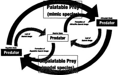
Thepredatorcannotdistinguish the mimic from themodel,sothat eachpredatorsearches and attacks

them withcommonprobability. Once apredator predates a model individual, itcomes to omit both the

model and the mimic species from its diet menu, and then not to search nor attack them in the

same

day. Ifapredator predates amimic individual, it comesto increase the search and attack probability for

the model and the mimic. Thepredator population size is assumed to be kept constant, independently

of the model and themimic population sizes. The frequency ofpredatorswith higher search-and-attack

probability and thatwithzerosearch-and-attack probability decreasesbyarate between thesubsequent

days,because ofthe predator$s$losingthesearch image. Analyzingourmodelsystem, wecangetthe result

suchthat the conditionforthepersistenceof modelpopulationdoes not depend on the mimicpopulation

size, while the conditionforthepersistence ofmimicpopulation doesdepend onthepredator$s$ability of

Figure1: Multi time-scalestructureofpopulationdynaniicsinourmodel.

Figure 2: Pradator$s$state transition due to predating themodelorthe mimicprey.

2

Model

Weanalyzeamathematical model consisting of the daily populationdynamicswithordinarydifferential

equations, the seasonal population dynamics with difference equations, and the annual population

dy-namics withdifferenceequations (seeFig. 1). Eachpredationseason iscomposedwith the dailydynamics

repeatedday by day in$T$days.

Thepredator populationsizeisassumed to bekept constant, given by$P$, independently ofthe model

and themimicpopulationsizes. This

means

suchanassumptionthat thepredatorisageneralistandhas

someother preys tokeep the stationary population size, sothatitcansurvive andsustain itspopulation

evenif the model and the mimic population go extinct.

The reproductions of model,mimic, andpredator speciesis assumed to

occur

between the subsequent

predation

seasons.

In otherwords, thereisnoreproduction ofmodel, mimicor predatorwithin the

pre-dation season,sothat the model and the mimicpopulationsmonotonicallydecrease due to thepredation

Daily dynamics

Thepredator cannot distinguish the mimic $hom$the _model,so _{that each predatorsearches and attacks}

themwith

common

probability. Once

a

predator predates

a

modelindividual, it

comes

toomitboth the

model and the mimic species from its diet menu, and then not to search nor attack them in the same

day. Ifapredator predatesamimic individual, it comesto increase the search-and-attack probability for

both the model and the mimic (see Fig. 2).

At the predation period in the $k$ th day ofpredation season, the predator subpopulation without

any search image for the model/mimic prey is now given by $P_{k}^{0}(t)(k=1,2, \ldots,T)$, at time $t$ after

the beginning of the predation period $(t=0)$

.

In the

same

way, the predator subpopulation with

higher search-and-attack probability after predating a mimic prey is given by $P_{k}^{+}(t)$, and that with

zero probability after predating amodel prey by $P_{k}^{-}(t)$

.

From the assumption ofa constant predator

population size,

$P_{k}^{0}(t)+P_{k}^{+}(t)+P_{k}^{-}(t)=P$

for any $t\in[0, \tau]$, where $\tau$ is the length of predation period in which the daily dynamics undergoes

in

each day. The model and the mimic populationsizes at time$t\in[0, \tau]$ in thedaily dynamics

are

given

by$m_{k}(t)$ and$x_{k}(t)$.

In

our

model,thedaily dynamicsis governedby the following ordinary differential equations:

$\frac{dm_{k}(t)}{dt}$ $=-F_{M}^{0}P_{k}^{0}(t)-F_{M}^{+}P_{k}^{+}(t)$; $\frac{dx_{k}(t)}{dt}$ _{$=-F_{X}^{0}P_{k}^{0}(t)-F_{X}^{+}P_{k}^{+}(t)$}; $\frac{dP_{k}^{0}(t)}{dt}$ $=-F_{M}^{0}P_{k}^{0}(t)-F_{X}^{0}P_{k}^{0}(t))$ (1) $\frac{dP_{k}^{+}(t)}{dt}$ $=F_{X}^{0}P_{k}^{0}(t)-F_{M}^{+}P_{k}^{+}(t)$; $\frac{cfP_{k}^{-}(t)}{dt}$ _{$=F_{M}^{0}P_{k}^{0}(t)+F_{\#\backslash 1}^{+}P_{k}^{+}(t)$},

where $\Gamma_{M}^{0}\langle$ is the predationrate for the model perunit population

size of$P_{k}^{0}(t)$ at time$t$, and the others

aredefined

as

well, which

are

nowgiven by

$F_{M}^{0}=\mu_{k}(t)\cdot b_{0}\{m_{k}(t)+xk(t)\}$; $F_{M}^{+}= \mu_{k}(t)\cdot\frac{b_{0}}{c+}\{m_{k}(t)+x_{k}(t)\}$; $F_{X}^{0}=\chi_{k}(t)\cdot b_{0}\{m_{k}(t)+x_{k}(t)\}$; $F_{X}^{+}= \chi_{k}(t)\cdot\frac{b_{0}}{c+}\{m_{k}(t)+x_{k}(t)\}$

with

$\mu_{k}(t)=\frac{m_{k}(t)}{m_{k}(t)+x_{k}(t)}$; $\chi_{k}(t)=\frac{x_{k}(t)}{mk(t)+x_{k}(t)}$.

Parameter $b_{0}$ isthe predation coefficient of the predator which doesnot experiencethepredation of the

model and the mimic preys. The contact rateofapredator_{with preys is assumed to be} proportionalto

thesumofmodel and mimicpopulations, $m_{k}(t)+x_{k}(t)$. Parameter$c^{+}$ is positiveand less than 1, which

gives the increaseof predationrate bythe creation of search image due to the predationof the mimic

prey.

Makinguseofthe following non-dimensionalizing parametertransformation:

the system (1) becomes $\frac{dm_{k}(t)}{dt}$ $=-P \{p_{k}^{0}(t)+\frac{p_{k}^{+}(t)}{c+}\}m_{k}(t)$; $\frac{dx_{k}(t)}{dt}$ $=-P \{p_{k}^{0}(t)+\frac{p_{k}^{+}(t)}{c+}\}x_{k}(t)$; $\frac{dp_{k}^{0}(t)}{dt}$ _{$=-\{m_{k}(t)+x_{k}(t)\}p_{k}^{0}(t)$}; (2) $\frac{dp_{k}^{+}(t)}{dt}$ $=p_{k}^{0}(t)x_{k}(t)- \frac{p_{k}^{+}(t)}{c^{+}}m_{k}(t)$; $\frac{dp_{k}^{-}(t)}{dt}$ _{$= \{p_{k}^{0}(t)+\frac{p_{k}^{+}(t)}{c+}\}m_{k}(t)$}.

Now$p_{k}^{0},$$p_{k}^{+}$ and$p_{k}^{-}$ respectivelymeanthe frequency of predatorsaccording to the state characterized by

thesearch-and-attack probability, satisfyingthat

$p_{k}^{0}(t)+p_{k}^{+}(t)+p_{k}^{-}(t)=1$

for any$t\in[0, \tau]$.

Seasonal

dynamics

The model and the rnimicpopulation sizes at the end of$k$th predation period inthepredation season

are

givenby$m_{k}(\tau)$ and$x_{k}(\tau)$

.

They givethe initial populationsizes in the subsequent predation period

ofthe next day: $(m_{k+1}(0), x_{k+1}(0))=(m_{k}(\tau), x_{k}(\tau))$. We ignore the death rate due to any other

reasons

except for the predationinevery day ofthe predation

season.

As for the frequencies in the predator population, we introduce the probabilityoflosing the search

image, say,theforgetting probability. Thepredator losesits searchimage with aprobabilitybetween the

end ofapredation period and the beginningofthe subsequent predation period. Thepredator withthe

highersearch-and-attack probabilityloses itwithprobability $1-\sigma^{+}$,where$\sigma^{+}$ meansthe probabilityto

keep_{the attractive search}image$(0\leq\sigma^{+}\leq 1)$

.

$\ulcorner\Gamma he$predatorwith thelower search-and-attackprobability

loses it with probability $1-\sigma^{-}(0\leq\sigma^{-}\leq 1)$. So the parameter $\sigma^{-}$

means

the probability tokeep the

repulsivesearch im\‘age. Therefore, we

assume

the relation between the predatorfrequencies at the end

of$k$thpredation period and those at thebeginning of$k+1$ thone asfollows:

$p_{k+1}^{0}(0)$ $=p_{k}^{0}(\tau)+(1-\sigma^{+})p_{k}^{+}(\tau)+(1-\sigma^{-})p_{k}^{-}(\tau)$;

$p_{k+1}^{+}(0)$ $=\sigma^{+}p_{k}^{+}(\tau)$; (3)

$p_{k+1}^{-}(0)$ $=\sigma^{-}p_{k}^{-}(\tau)$.

Hence, ifthe model and the mimicpopulations donotexistor goesextinct, the frequency$p^{0}$

asymptoti-cally approaches 1 day by day in ageometric manner. Theseboundary conditionsfor the model/mimic

populations andthe predator frequenciesgovem theirseasonal dynamics througheach predationseason

of$T$days.

Annual

dynamics

Letus consider the$n$th predation

season.

The initial population sizes of model and mimic

are

given by

$m_{1}(0)$and$x_{1}(0)$from thedefinitions for thedailydynamics. These initialpopulationsizessimultaneously

define the initial population sizes for the$n$ th predation season, now rewritten by_{$M_{n,0}(=m_{1}(0))$} and

$X_{n,0}(=x_{1}(0))$

.

In our model, the reproduction of the model and the mimic populations is given by what is called

Beverton-Holt model. Since the reproduction season is now assumed to be between subsequent pre

$(M_{n+1,0}, X_{n+1,0})=(m_{1}(0),x_{1}(0))$ at the beginning of$n+1$th predation

season:

$M_{n+1,0}$ $= \frac{r_{M}m_{T}(\tau)}{1+\beta_{M}m_{T}(\tau)}$

.

(4)

$X_{n+1,0}$ $= \frac{r_{X}x_{T}(\tau)}{1+\beta_{X}x_{T}(\tau)}$,

where $r_{M}$ and $r_{X}$

are

respectivelythe intrinsic growthrate,$\beta_{M}$ and$\beta_{X}$ the density effect coefficient.

In

our

model,we

assume

that the predator completely loses the search image in the period between

subsequent predationseasons. Thus the initial condition forthe predator$s$ frequencies accordingto the

stateofsearch-and-attackprobability is given by

$(p_{1}^{0}(0),p_{1}^{+}(0),p_{1}^{-}(0))=(1,0,0)$,

onthe first day ofany predationseason,independently of theirvalues at the end of previousseason.

3

Analysis

Daily dynamics

From(2), we caneasilyfind that $d(\log m_{k})/dt=d(\log x_{k})/dt$_{for any}$t\in[0, \tau]$. This

means

that theratio

$Xk(t)/mk(t)$isconstant independently of$t$, sothat $x_{k}(t)/m_{k}(t)=Xk(0)/m_{k}(0)$for any_{$t\in[0, \tau]$} and any

$k=1,2,$$\ldots,$$T$. Moreover, from the boundary condition $(m_{k+1}(0),x_{k+1}(0))=(m_{k}(\tau)_{)}x_{k}(\tau))$, we lastly

have

$\frac{x_{k}(t)}{m_{k}(t)}=\frac{x_{k}(0)}{m_{k}(0)}=u_{n}:=\frac{ir_{1},(0)}{m_{1}(0)}$ (5)

for any $t\in[0, \tau]$ and any $k=1,2,$_$\ldots,$$T$ in the $n$ th predation season. We remark that, from the

definition,$x_{1}(0)/m_{1}(0)=M_{n,0}/X_{n,0}$, the ratio atthe beginningof the first predation period in the$n$th

predationseason. Furthermore, from (2),we can find that $d(m_{k}+p_{k}^{-}P)/dt=0$ for any $t\in[0, \tau])$ too.

Thus, we have

$m_{k}(t)=m_{k}(0)-\{p_{k}^{-}(t)-p_{k}^{-}(0)\}P$ (6)

for any $t\in[0, \tau]$.

Now, from (2),since$dm_{k}/dt<0$forany$p_{k}^{0}>0,$$p_{k}^{+}>0$and$m_{k}>0,$$m_{k}(t)$ismonotonically decreasing

in terrnsof$t\geq 0$. On the otherhand, $\prime n_{k}(t)\equiv 0$is aspecificsolution for the first differential equation

of (2). Thus, becauseofthe uniqueness of solution, $m_{k}(t)$ with any positive initial value _{$m_{k}(0)>0$} is

bounded from below. Therefore, $\lim_{tarrow\infty}m_{k}(t)=m_{k}^{*}\geq 0$ exists. Fkom (2) with the trivial boundedness

such that$p^{-}\leq 1$, makinguseofthe analogous arguments,wefind that

$\lim_{tarrow\infty}p_{k}^{-}(t)=p_{k}^{-}"$ $\geq 0$exists, too.

Lastly, thismeansthat $\lim_{tarrow\infty}p_{k}^{+}(t)=p_{k}^{+*}\geq 0$ and $\lim_{\dagger.arrow\infty}p_{k}^{0}(t)=p_{k}^{0*}\geq 0$exist at thesame time.

If$m_{k}^{*}>0$, then, from (2),it is necessary that$p_{k}^{0*}=p_{k}^{+*}=0$ sothat$p_{k}^{-}‘$ $=1$. In this case, from (6),

$m_{k}^{*}=m_{k}(0)-\{1-p_{k}^{-}(0)\}P$,which is validwhenandonlywhen$mk(0)>\{1-p_{\overline{k}}(0)\}P$

.

In contrast, from

(6), if$m_{k}^{*}=0$, then$p_{k}^{-}"$ $=p_{k}^{-}(0)+m_{k}(0)/P$which is valid when and only when _{$p_{\overline{k}}(0)+m_{k}(0)/P\leq 1$},

that is, $mk(0)\leq\{1-p_{k}^{-}(0)\}P$. In this case, from (5), $\lim_{tarrow\infty}xk(t)=x_{k}^{*}=0$ as well.

With these arguments, nowwe have thefollowingresult:

In the daily dynamicsgiven by (2), thesystem asymptotically approachesthe equilibriumstate

given by

$(m_{k}(t), x_{k}(t),p_{k}^{0}(t),p_{k}^{+}(t),p_{k}^{-}(t))arrow$$tarrow\infty\{\begin{array}{l}E_{0}(0,0,p_{k}^{0*},p_{k}^{+*},p_{k}^{-*}) if m_{k}(0)\leq\{1-p_{k}^{-}(0)\}P;E_{+}(m_{k}^{*}, u_{n}m_{k}^{*}, 0,0,1) if m_{k}(0)>\{1-p_{k}^{-}(0)\}P\end{array}$ (7)

Equilibrium

state

approximation

Now,weintroduceanapproximation for thestate atthe end of predation period. Let

us

assume

thatthe

state $(m_{k}(t),x_{k}(t),p_{k}^{0}(t),p_{k}^{+}(t),p_{k}^{-}(t))$approaches theequilibrium stategiven by (7) sufficiently fast. In

otherwords,

we

assume

that thestate at the end ofpredation period $(m_{k}(\tau),x_{k}(\tau),p_{k}^{0}(\tau),p_{k}^{+}(\tau),p_{k}^{-}(\tau))$

is sufficientlynear the equilibrium state givenby (7). Thus,

as an

approximation, wehereafter

use

the

equilibriumstategiven by (7) asthestate atthe end of predation period.

With this approximation, we reset up the relation between the predator frequenciesat the end of $k$

th predation period and those at the beginning of$k+1$ thone

as

follows $(k\geq 1)$:

$p_{k+1}^{0}(0)$ $= \lim_{tarrow\infty}\{p_{k}^{0}(t)+(1-\sigma^{+})p_{k}^{+}(t)+(1-\sigma^{-})p_{k}^{-}(t)\}$;

$p_{k+1}^{+}(0)$ $= \lim_{tarrow\infty}\{\sigma^{+}p_{k}^{+}(t)\}$; (8)

$p_{k+1}^{-}(0)$ $= \lim_{tarrow\infty}\{\sigma^{-}p_{k}^{-}(t)\}$,

insteadof (3).

From (7) and (8),

as

far

as

the mimic populationpersists and the system asymptotically approaches

the equilibrium state $E+$ in the$k$ th predation period,

we

have

$(p_{k+1}^{0}(0),p_{k+1}^{+}(0),p_{k+1}^{-}(0))=(1-\sigma^{-}, 0, \sigma^{-})$

.

In contrast,

once

the mimicpopulation goes extinct in the$k$ th predation periodwith the equilibrium

state$E_{0}$ in (7),which could be regarded

as

theconsequenceof predator‘sovergrazing,

we

have

$p_{k+1}^{0}(0)$ $=p_{k}^{0*}+(1-\sigma^{+})p_{k}^{+\prime}+(1-\sigma^{-})p_{k}^{-}.$;

$p_{k+1}^{+}(0)$ $=\sigma^{+}\rho_{k)}^{+}$

$p_{k+1}^{-}(0)$ $=\sigma^{-}p_{k}^{-}.$.

Subsequently, since the mimic and the model populations have gone extinct, the system (2) gives no

changeofthepredator frequencies in the subsequentpredation period. Thus, wehave

$p_{k+1}^{0}$ $=p_{k}^{0*}+(1-\sigma^{+})p_{k}^{+*}+(1-\sigma^{-})p_{k}^{-*}$;

$p_{k+1}^{+*}$ $=\sigma^{+}p_{k}^{+*}$;

$p_{k+1}^{-*}$ $=\sigma^{-}p_{k}^{-*}$.

Therefore,thepredator frequenciesgeometricallyapproach $(1, 0,0)$day by day after the extinction of the

mimic and the model populations, because ofthepredator$s$losing thesearch image.

Now,suppose that the mimicpopulation persiststill the$k$thpredation period. Then, fromthe above

arguments,

we

have $(p_{k}^{0}(0),p_{k}^{+}(0), p_{k}^{-}(0))=(1-\sigma^{-}, 0, \sigma^{-})$ for$k>1$

.

Further, from (2) and (5),

we

find that

$\frac{d}{dp_{k}^{0}(t)}[\frac{p_{k}^{+}(t)}{\{p_{k}^{0}(t)\}^{\alpha}}]=-\frac{u_{n}}{1+u_{n}}\frac{1}{\{p_{k}^{0}(t)\}^{\alpha}}$,

where$\alpha_{\mathfrak{n}}$$:=1/\{c^{+}(1+u_{n})\}$. Hence,we canobtainthefollowingrelation between$p_{k}^{0}(t)$ and $p_{k}^{+}(t)$ inthe

$k$thpredation period:

$p_{k}^{+}(t)=\{\begin{array}{ll}-(1-c^{+})p_{k}^{0}(t)\log\frac{p_{k}^{0}(t)}{p_{k}^{0}(0)} if \alpha_{n}=1;\frac{1}{\alpha_{n}-1}\frac{u_{n}}{1+u_{n}}p_{k}^{0}(t)[1-\{\frac{p_{k}^{0}(t)}{p_{k}^{0}(0)}\}^{\alpha_{\mathfrak{n}}-1}] if \alpha_{n}\neq 1.\end{array}$

Making

use

ofthisequationwith$p_{k}^{+}(t)=1-p_{k}^{-}(t)-p_{k}^{0}(t)$and$p_{k}^{+}=1-p_{k}^{-}"$ $-p_{k}^{0*}$,wecaneasilyprove

that theequilibrium state$E_{0}$ in (7) uniquelyexists with$0<p_{k}^{0}<1,0<p_{k}^{+*}<1$and _{$0<p_{k}^{-*}<1$}

.

(a)

(b)

Figure3: A numerical example of the seasonal dynamics governed by (2) with the equilibriumstateapproximation

(8). Solid curves show the daily dynamics, and dashed curves do the interval between subsequent predation

periods. (a) $(m_{1}(0), x_{1}(0))=$ (52.4469, 26.2234); (b) $(m_{1}(0), x_{1}(0))=$ (26.2234, 13.1117). Commonly, _$T=50$,

$\tau=2.0,$ $c^{+}=0.1,$ $\sigma^{+}=0.5,$ $\sigma^{-}=0.1,$ $P=1.0,$ $rr\iota_{c}=45.i$. The mimic and the model populations _persist

throughthepredation sea.sonin (a),whilethey goextincton aday ofitin (b).

Themimi$c$ and themodelpopulations persist inthe$k$ th predation penod

if

andonly

if

_{$m_{k}(0)>$}

$(1 -\sigma^{-})P$

for

$k>1$ and$m_{1}(0)>P.$ Then, $(p_{k}^{0*},p_{k}^{+*},p_{k}^{-*})=(0,0,1)$ and_{$m_{k}^{*}=m_{k}(0)-$}

$(1 -\sigma^{-})P$.

for

$k>1$ and_{$mi=m_{1}(0)$} –P.

If

and only

if

$m_{k}(0)\leq(1-\sigma^{-})P$

for

some

$k>1$ or$m_{1}(0)\leq P$, the mimic and the modelpopulations go extinct in the $k$ th or the

first

predationperiod, and then the system approaches the equilibrium state $E_{0}$ with$0<p_{k}^{0*}<1$,

$0<p_{k}^{+*}<1$ and$0<p_{k}^{-*}<1$.

As for aspecial case without the model population, when the system contains the mimic and the

predator,wecaneasilyshown that the mimicpopulationgoes extincton the

_first

day

_of

predation

season

with the equilibnum state approximation without the modelpopulation.

Seasonal

dynamics

Letusconsider thecasethat the mimic and themodel populations persist tillthe $k$ th predation period

$(k>1)$. Then, fromtheabovearguments withtheequilibriumstate approximation,wehave thefollowing

dailyrecurrence relation about theinitial model population size:

for $j=1,2,$$\ldots,$$k-1$. Since$p_{1}^{-}(0)=0$ and $p_{j}^{-}(0)=\sigma^{-}$ for $j>1$ , this

recurrence

relation gives the

following general form of$m_{j}(0)$:

$m_{j}(0)$ $=$ $m_{1}(0)-\{1+C-2)(1-\sigma^{-})\}P$ for$j=2,3,$$\ldots,$$k$

.

(10)

As

a

consequence,since thenecessaryandsufficientcondition that the mimic and the model populations

persist in the $T$ th predation period ($=$ thelast predation period in the predation season) is given by

$m_{T}(0)>(1-\sigma^{-})P$from theresult in the previoussection,wehave thefollowingresult about the seasonal

dynamics:

The mimic and themodelpopulations persest through the$n$ th predatior}

season

if

and only

if

$m_{1}(0)=M_{n,0}>m_{c}:=\{1+(T-1)(1-\sigma^{-})\}P$. (11)

Othemrise, the mimic and the model populationssimultaneouslygo extinct in the$k_{c}$ th day$0\int$

the$n$ th predation season, where the day $k_{\epsilon}$ the extinction occurs is determinedby

$k_{e}= \min\{j|j\geq\frac{M_{n,0}/P-1}{1-\sigma^{-}}+1,1\leq j\leq T\}$

.

(12)

In the

case

that the mimic and the model populations persist through the$n$ th predation season, the

mimic populationsize$m_{T}$ attheend of thepredation

season

is given by

$m_{\dot{T}}$ $=$ $m_{T}(0)-(1-\sigma^{-})P=m_{1}(0)-\{1+(T-1)(1-\sigma^{-})\}P$

$=$ $M_{\mathfrak{n},0}-m_{c}$. (13)

Asaconsequence, the extinction of onlyoneof mimic and modelnever

occurs

in theseasonaldynamics

of

our

model with the equilibriumstateapproximation, while it is likely that both of themgoextinct in it.

A numericalexampleoftheseasonaldynamicsgoverned by (2)with theequilibriumstateapproximation

(8) is given in Fig. 3.

Annual dynamics

From (4) with the equilibrium state approximation (8), the model and the mimic populations at the

beginning of$n+1$ th predation season,$M_{n+1,0}$ and$X_{n+1,0}$, are nowgiven by the following reproduction

functions: $M_{n+1,0}$ $= \frac{r_{M}m_{\dot{T}}}{1+\beta_{M}m_{T}}$; (14) $X_{n+1,0}$ $= \frac{r_{X}x_{T}^{*}}{1+\beta_{X}x_{T}^{*}}$, where $x_{T}^{*}=u_{n}m_{T}^{*}= \frac{x_{1}(0)}{m_{1}(0)}m_{T}^{*}=\frac{X_{n,0}}{M_{n,0}}m_{J’}^{*}$,

from (5). Then, from (7), (11), (13) and (14), we have the following difference equations todetermine

the annualdynamics in termsofthe model and the mimicpopulationsizes at thebeginningofpredation

season:

$M_{n+1.0}$ $= \frac{r_{M}[M_{\mathfrak{n},0}-m_{c}]_{+}}{1+\beta_{M}[M_{n,0}-m_{c}]_{+}}$;

(15)

$X_{n+1,0}$ $= \frac{r_{X}[M_{n,0}-m_{c}]_{+}X_{n,0}}{M_{\iota,0}+\beta_{X}[M_{\iota,0}-m_{c}]_{+}X,,0}$,

where the symbol $[$ $]_{+}$ is definedby

Wenotethat the annual dynamics of model population is independent ofthatofmimic population, while

thelatterdepends

on

the former.

Analyzing the first equationof(15),

we

can

obtain thefollowing resultaboutthepersistenceofmodel

population:

If

and only

_if

the following conditions are satisfied, the model population persists in any

predation season, and$M_{n,0}arrow M^{*}=m_{c}+\lambda+=(r_{M}-1-m_{c}/\lambda_{+})/\beta_{M}$ as$narrow\infty$:

$r_{M}$ $\geq$ $(1+\sqrt{\beta_{M}m_{c}})$

.

; (16) $M_{1,0}$ $\geq$ _{$m_{c}+\lambda_{-}=(r_{M}-1-m_{c}/\lambda_{-})/\beta_{M}$}, (17) where $\lambda\pm=\frac{1}{2\beta_{M}}[r_{M}-(1+\beta_{M}m_{c})\pm\sqrt{\{r_{M}-(1+\sqrt{\beta_{M}m_{c}})^{2}\}\{r_{M}-(1-\sqrt{\beta_{M}m_{c}})^{2}\}}]$

.

(18)

Othemrise, the modelpopulationgoes extinct in the$n_{e}$ th predation

season

with$M_{n_{*},0}\leq m_{c}$,

where

$n_{\epsilon}$. $=1+[ \frac{\log(\frac{1-[M_{n,O}-m_{c}]_{+}/\lambda+}{1-[M_{n,O}-m1+/\lambda-})}{\log(\frac{1+\beta_{M}\lambda_{+}}{1+\beta_{M}\lambda_{-}})}I\cdot$ (19)

The symbol$[x$

I

means

the smallestintegernot less than$x$.

As for themimicpopulationgovernedbythe second differenceequationof(15), here letusconsider it

with$M_{n,0}\equiv M^{*}=m_{c}+\lambda+$ for any$n$

.

This is because the model population dynamics is independent of

themimic one. Besides, as wehave already seen, if the model population goesextinct, thenso does the

mimicpopulation. Further, we canprovethat,even ifthemimicryis absent, theseasonalandtheannual

dynamics for the model populationisthesame as shown above. Sowenow focus the mimic population

dynamicswhen themodel populat,ionhas reachedit,$s$equilibriumstateaccordingtothe annual dynamics

governedby thefirst differenceequation of (15). Hence, instead ofthe second differenceequationof(15),

let usconsider here the following annual dynamics of mimicpopulation:

$X_{n+1,0}= \frac{r_{X}X_{n,0}}{1+m_{c}/\lambda_{+}+\beta_{X}X_{n,0}}$. (20)

$\mathbb{R}om$this differenceequation,we obtain the followingresult about thepersistence

of mimic population:

If

and only

_if

the following condition is

_satisfied

when the model population persists at its

equilibnum state, the mimic populationpersists in anypredation

season:

$r_{X}>1+ \frac{m_{c}}{\lambda_{+}}=r_{M}-\beta_{M}M^{*}$, (21)

and then

$X_{n,0} arrow X^{*}=\frac{1}{\beta_{X}}\{r_{X}-(1+\frac{m_{c}}{\lambda+})\}=\frac{\beta_{M}}{\beta_{X}}M^{*}+\frac{?^{\backslash }x-r_{M}}{\beta_{X}}$ (22)

as$narrow\infty$. Otherwise, the mimic populationgoes extinct, that is, $X_{n,0}arrow 0$ as$narrow\infty$

for

any$X_{1,0}>0$

.

Differently from the case ofmodel population, thereis nocondition for the initial value$X_{1,0}$ about the

mimic population persistence.

We note that, in thisresult, unless the condition (21) issatisfied, the mimic populationtends to go

extinct, though its extinction never

occurs

at any finite time as long

as

the model population persists.

Asalreadyseenin the seasonal dynamics, the mimicpopulation goes extinct inapredation

season

only

whensodoes themodel population. Thus, the mimic’sextinctioninthe above resultmeansthe tendency

for the mimicpopulationto goextinct. In suchcase, the mimic populationsize decreases not onlyday

by day in the predationseason but also yearby year, independently ofthe temporal variation ofmodel

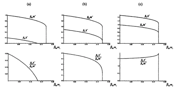
(a) (b) (c)

Figure 4: m.-dependenceofequilibrium population sizes atthe beginningof predationseason, that is, forthe

annual dynamics of (2) and (14) with the equilibriumstate approximation (8). (a) $rx=1.2;(b)rx=1.5;(c)$

$r_{X}=2.5$

.

Commonly, $r_{M}=2.0$. In caeeof (a), themimic population is extinct fora range of$m_{c}$ inwhich the

model population is persistent. Incasesof(b) and(c), themimicpopulationis persistent as longasthe model

population is.

Equilibrium

population

size ratio

Inthecasewhen the modelpopulationispersistentunderthose conditions(16)and (17), then, from (5),

we can show that the ratio of theirpopulation sizes approaches aconstant at any moment in the daily

dynamics ofany predationseason:

$\frac{X_{n,0}}{M_{n,0}}=\frac{x_{k}(t)}{m_{k}(t)}=u_{n}arrow\frac{X}{M^{*}}=\frac{\beta_{M}}{\beta_{X}}\cdot\frac{[r_{X}-1-m_{c}/\lambda_{+}]_{+}}{r_{M}-1-m_{c}/\lambda_{+}}$ (23)

as $narrow\infty$, where $[$ $]_{+}$ is defined as before. Numerical examples of_{$m_{c}$}-dependence ofthe equilibrium

populationsizeratio aregiven in Fig. 4.

Wecaneasily find that $m_{c}/\lambda_{+}$ is monotonically increasing and$m_{c}+\lambda_{+}$ is monotonically decreasing

in terms of $m_{c}$. Since $m_{r}$, defined in (11) is monotonically decreasing between its minimum $P$ and

maximum $TP$ in terms of $\sigma^{-}$, the results ofour analysis indicate that the persistence of model and

mimicpopulation depends on thepredator$s$ ability of repulsivesearchimageformation. Moreover, it is

likely that thepredator‘sabilityofrepulsivesearchimageformation could determine thepopulation size

ratiobetween themimic and the model populations.

4

Concluding Remarks

As the predator‘s ability ofrepulsive search image formation is better, it is more likely for the model

population to persist, andthe

equilibri.um

model population size gets larger. This isbecause the better

ability ofrepulsive search image formation indicates to repel the predator from the model population

so

as

to make the predation praesure weaker for it. This feature according to the predator‘s ability of

repulsive search image formation can be adopted to the persistence and the equilibrium size of mimic

population,too. At thesametime, this result impliesthat theequilibrium populationsize ratiobetween

themodel and the mimic is affected bythepredator’s ability of repulsivesearch imageformation.

Beyondtheseresultsin thepopulation dynamical nature, wecould extendour resultto some

discus-sionsonthe evolution or the invasion ofmimicry from theviewpointof coexistenceofthemimicand the

model populations. Iiurther, wecould discuss the possible_{coevolutionary relation between the} predator